The neural-nets-as-a-distributed-system track has been building one object in simulation — the traffic matrix $M_{ij}$, the bytes device $i$ sends device $j$ in a step. Collectives populate it, consistency relaxes when it settles, MoE routing makes it a function of the input. This post is about the two things you actually do with $M_{ij}$ on a real cluster: measure it, and decide the network that carries it.
The old way, and what changed
For years the workflow for "why is my all-reduce slow" was NCCL_DEBUG=INFO,
grep, and eyeball. No structured per-peer data. That changed when NCCL 2.23
shipped a real profiler-plugin API; the NCCL Inspector plugin (matured in
2.28) turns it into low-overhead, per-communicator, per-collective JSON you can
actually pivot into a heatmap. Turn it on with:
export NCCL_PROFILER_PLUGIN=.../libnccl-profiler-inspector.so
export NCCL_INSPECTOR_ENABLE=1
export NCCL_INSPECTOR_ENABLE_P2P=1        # peer-to-peer (pipeline) tracking
export NCCL_INSPECTOR_DUMP_DIR=/path/to/logs
and every collective drops a record like this:
{"header":   {"id": "0x7f8c49...", "rank": 2, "n_ranks": 8, "nnodes": 1},
 "coll_perf":{"coll": "AllReduce", "coll_msg_size_bytes": 17179869184,
              "coll_exec_time_us": 61974, "coll_busbw_gbs": 485.12}}
The catch: Inspector is per-communicator, not per-peer
Here is the subtlety that makes reconstructing $M_{ij}$ an actual technique
rather than a jq one-liner. That record tells you how much rank 2 moved in
communicator 0x7f8c49… and how fast — but not which peer received it. An
all-reduce is a group operation; there is no destination field. So a rank×rank
matrix needs two ingredients Inspector does not give you directly:
- The layout — which global ranks form each communicator. You build this
from your parallelism config; in Prometheus mode Inspector even labels the
communicators
"DP Group 0","TP Group 1", which is the hint you need. - The algorithm — a ring all-reduce over $k$ ranks puts $\frac{2(k-1)}{k}\times \text{bytes_per_rank}$ on each ring-neighbor link. That is what attributes a rank's aggregate volume onto specific peer links.
Join Inspector's volumes with the layout and overlay the ring, and the matrix appears. Here it is for a synthetic-but-schema-accurate 8-GPU, 2-node job running tensor-parallel within each node and data-parallel across them:
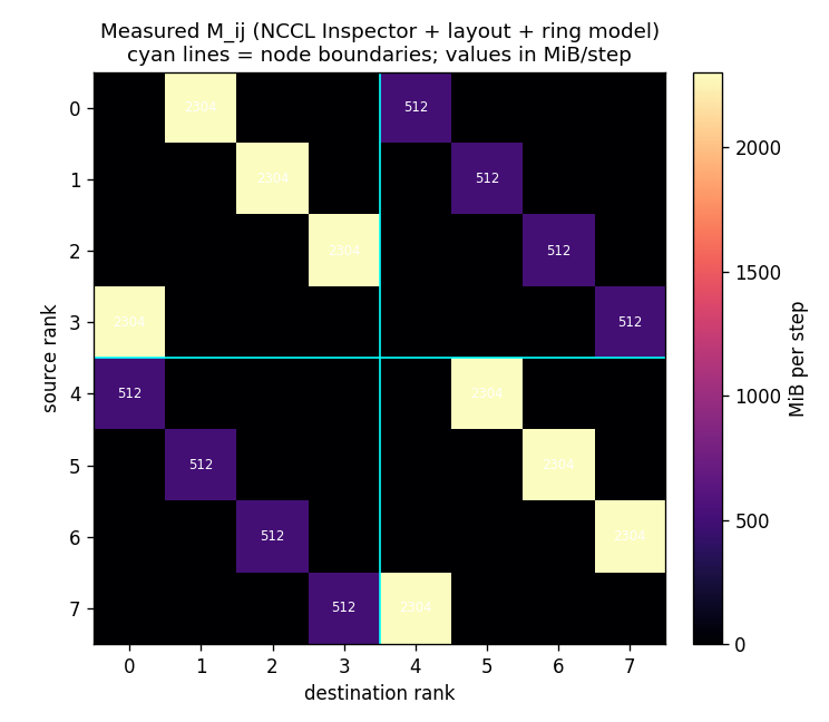
The structure is the whole story. Bright intra-node TP rings (2304 MiB on each
neighbor link — tensor parallel runs an all-reduce inside every layer) and thin
inter-node DP links (512 MiB — one gradient all-reduce per step). And notice
where the cross-node links sit: 0↔4, 1↔5, 2↔6, 3↔7 — every
data-parallel pair is the same GPU index on different nodes. That is not an
accident; it is what "on-rail" means, and it is about to decide the hardware.
The fabric decision falls out of the structure
A rail-optimized network exploits exactly that observation: same-index GPUs across nodes share a dedicated rail of cheap direct optics, and only traffic that must cross between rails uses an expensive rearrangeable spine. A fat-tree provisions full any-to-any bisection — it can carry anything, but you pay for the switching to do it.
So split inter-node traffic into on-rail (same index, cheap) and
cross-rail (different index, needs spine). The cross-rail fraction decides
everything. Provision a fat-tree to serve the job at cost 1.0, and a
rail-optimized fabric with a spine only 0.1 as large:
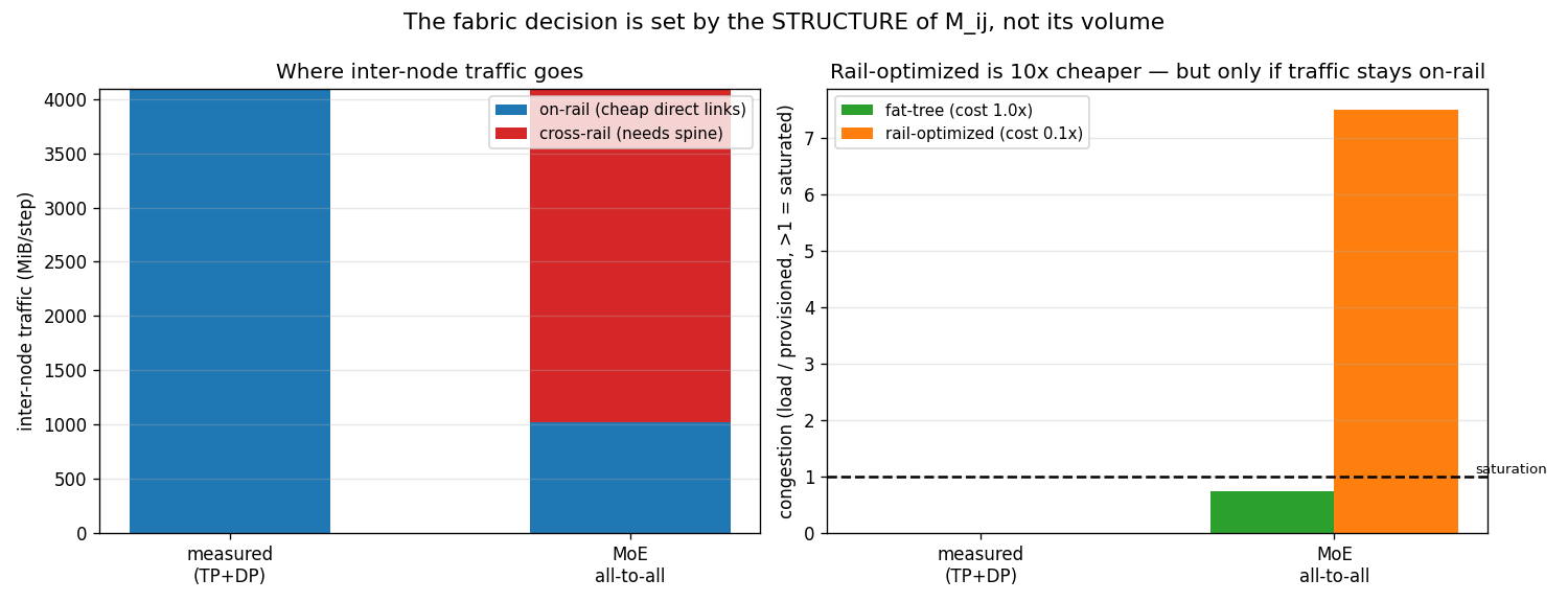
fabric decision (spine_fraction = 0.1, congestion > 1.0 = saturated):
  measured (TP+DP)   cross-rail frac=0.00  | fat-tree cong=0.00  | rail cong=0.00  -> rail VIABLE
  MoE all-to-all     cross-rail frac=0.75  | fat-tree cong=0.75  | rail cong=7.50  -> rail SATURATES
Same eight ranks, same inter-node volume. For the dense TP+DP job every
inter-node byte is on-rail, so the rail-optimized fabric carries it at zero
congestion for one-tenth the cost. Swap in an MoE all-to-all — identical volume,
but now spread across rails — and that same fabric is 7.5× oversubscribed;
now you must buy the fat-tree. The break-even is exactly
cross_rail_frac ≤ spine_fraction.
That is the sentence to leave with: the fabric decision is set by the structure of $M_{ij}$, not its volume. And it is why MoE changes the hardware conversation, not only the software one — a data-dependent topology that spreads across rails can invalidate a network that was perfectly sized for a dense model.
Why this matters for Megatron-scale jobs
- Observability first. If you cannot recover $M_{ij}$ from the running system, you are guessing. Inspector (per-collective bandwidth + P2P) is the default; Spectrum-X NetInspector adds fabric-level congestion; Meta's Holistic Trace Analysis builds comm heatmaps and straggler analysis from PyTorch/Kineto traces.
- Predicted vs observed. The measured $M_{ij}$ is the real-hardware version of what the MoE simulator produces. Comparing them is how you separate a routing problem (skew you can fix with the load-balancing loss) from a fabric problem (placement you fix in the topology).
- Co-design. Once you can see $M_{ij}$, the network becomes a design variable — rail-optimized, TopoOpt-style joint optimization, congestion-aware placement. Model it before you buy it with ASTRA-sim + Chakra.
Addendum: can MPI_T give a vendor-agnostic version of this?
A natural follow-up: instead of an NVIDIA-specific tool, could you build this on
MPI_T or the PMPI profiling interface and get a backend-neutral heatmap?
No — and the reason is instructive. NCCL is not an MPI implementation; its
collectives never call MPI_*, so PMPI's name-shifted wrappers intercept nothing,
and MPI_T only exposes counters internal to an MPI library. In a modern training
job MPI is usually just the bootstrap (rank exchange at init), while all the heavy
traffic flows through NCCL. An MPI_T/PMPI heatmap would therefore be nearly empty.
The agnostic layer has to live above the backend: normalize every source into
one record — {backend, comm, rank, coll, bytes, members} — and let the matrix
builder be backend-independent. I built exactly that with four adapters spanning
three totally different formats — structured JSON, unstructured debug logs, and
framework traces:
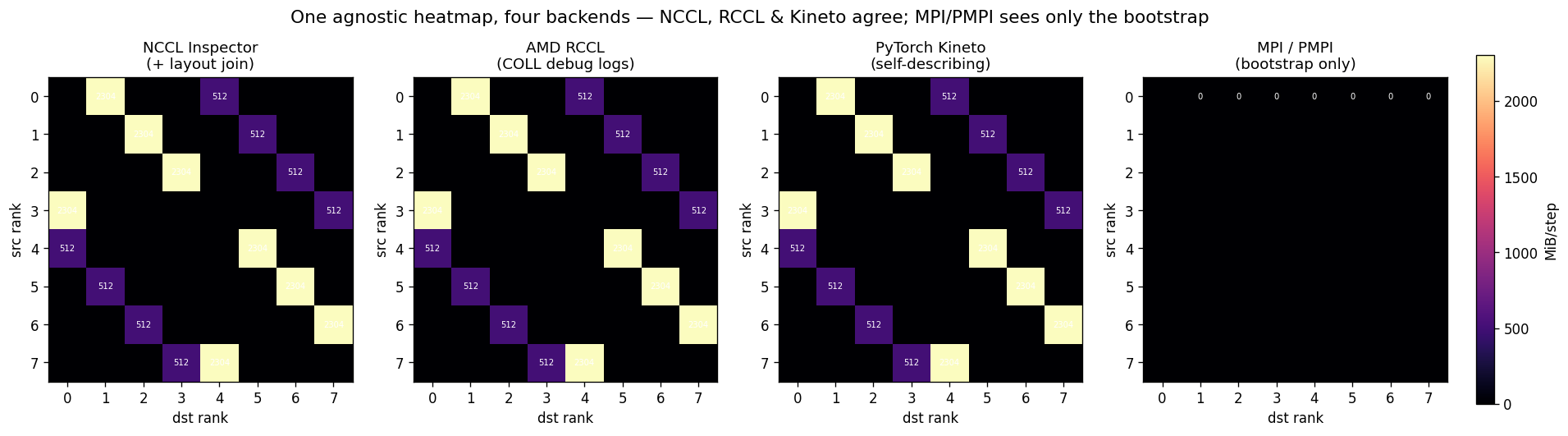
NCCL Inspector  :  200 ops,  16384 MiB payload, matrix sum 22528 MiB
AMD RCCL        :  200 ops,  16384 MiB payload, matrix sum 22528 MiB   <- identical
PyTorch Kineto  :  200 ops,  16384 MiB payload, matrix sum 22528 MiB   <- identical
MPI / PMPI      :    8 ops,      0 MiB payload, matrix sum     0 MiB   <- bootstrap only
NCCL Inspector, AMD RCCL, and PyTorch Kineto recover the identical
$M_{ij}$; the MPI/PMPI trace sees only the bootstrap. Each backend needs only a
thin adapter: Kineto is self-describing (its Process Group Ranks carries global
membership, so no external layout is needed — the framework-trace layer is the
most portable place to build this); RCCL is the messiest, since its
NCCL_DEBUG_SUBSYS=COLL logs carry no membership, so the adapter correlates the
INIT commHash lines with the COLL lines and gathers members as the union of
ranks per hash. MPI_T isn't the foundation; it's just one more thin adapter for
the MPI slice.
The full write-up with the parallelism taxonomy and the tooling landscape is in
the repo's discussion doc, and the runnable code — Inspector parser, layout join,
ring model, and the fabric evaluator — is
neural-nets/projects/04-observability-topology.
It runs on a laptop against a schema-accurate sample and is drop-in for a real
NCCL_INSPECTOR_DUMP_DIR.
Sources: NVIDIA — Enhancing Communication Observability with NCCL Inspector, NCCL Inspector plugin README, Real-Time Monitoring with NCCL Inspector and Prometheus.