In the previous post we treated the all-reduce contract as sacred: every worker sees the exact global average, every step. That makes the shared parameter linearizable — the strongest consistency you can ask for. It is also the source of the single most annoying failure mode in distributed training: the straggler tax. A barrier every step means the whole job runs at the speed of its slowest worker.
Distributed datastores hit this exact wall a decade ago and answered by weakening consistency. SGD turns out to have the same knob.
The knob
| model | rule | staleness | buys / costs |
|---|---|---|---|
| sync (BSP) | every update sees current weights | 0 | best progress-per-update, worst throughput |
| bounded-staleness (SSP) | a worker runs at most s steps ahead |
≤ ~s·N |
the dial between the two |
| async (ASP) | apply whatever you computed, whenever | unbounded | best throughput, staleness noise |
Bounded staleness — the Stale Synchronous Parallel model of Ho et al. (2013) — is the interesting middle. It is the database's "bounded staleness" consistency level, transplanted onto a gradient.
The experiment
N workers train a convex logistic-regression model in a single-process event simulator (NumPy only — it runs on a laptop). The one ingredient that makes any of this matter: worker 0 is a 4× straggler. Without stragglers you would just keep the barrier; with them, the barrier is a tax you want to escape.
Each worker computes its gradient on the weights it read. Other workers' updates
land before it finishes — and that gap is the staleness. The SSP gate simply
refuses to let a worker get more than s applied-steps ahead of the slowest one.
Running all four configurations to the same wall-clock budget:
consistency model       updates  updates/sec  mean stale  max stale  final loss
sync (BSP)                  105         0.26        0.00          0      0.2611
bounded s=2 (SSP)           855         2.13        3.53         14      0.2688
async (ASP)                2934         7.33        6.98         45      0.2672
Three things to take away
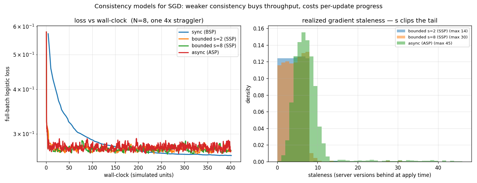
1. Hardware efficiency vs statistical efficiency. Async did ~28× the updates of sync in the same wall-clock — it never waits for the straggler. But each update is staler, so each makes less progress. Throughput and progress-per-update pull in opposite directions; total progress is their product, and that is what you actually optimize.
2. The bound s controls the tail, not the mean. With N workers in flight,
mean staleness floors near N no matter what s is — there are always ~N−1 other
updates in flight. What s clips is the maximum staleness (14 → 30 → 45 as
s goes 2 → 8 → ∞ in the full run). That tail is what destabilizes training at
high learning rates, which is exactly why you bound it rather than going fully
async.
3. Sync wins the asymptote; async wins early. Async and SSP drop fast while sync is still crawling behind the straggler — but the barrier buys sync a cleaner, lower final loss. Where you stop decides which one you would have picked. Short budget: relax consistency. Chasing the last decimal: keep the barrier.
Back to the fabric
This connects straight to the collectives post and to Megatron:
- Sync (BSP) is the data-parallel all-reduce path from post 12 — the linearizable barrier.
- The async / parameter-server path is what you reach for when stragglers or elastic membership make that barrier too expensive. It is the same motivation behind PS architectures and overlapped, relaxed gradient sync.
- Staleness here is a consistency relaxation. In the next post the topology itself becomes data-dependent (MoE routing). Different morph, same theme: the network bending to fit the workload instead of the other way around.
Code and the simulator:
neural-nets/projects/02-consistency.