This is the first hands-on post in the neural-nets-as-a-distributed-system track. We start where every scaled training run starts: the all-reduce.
The contract, not the algorithm
The single most useful reframing: an all-reduce is a contract, not an algorithm. The contract is "every rank ends holding the elementwise sum of every rank's input vector." How you realize that contract is open — and the cheapest realization changes with the situation. That changing is the whole point of this track.
We implement three realizations from scratch, each rank a real OS process, with point-to-point links modeled as queues. We don't measure wall-clock — process and pickle overhead would drown out the interconnect and tell you nothing. We measure the two quantities that do transfer to a real fabric:
- bytes-on-wire — total data moved, and whether it piles onto a hotspot;
- message rounds — the latency-bound critical path.
The three algorithms
Naive (gather → broadcast). Every rank ships its vector to rank 0; rank 0
sums and broadcasts the result back. Simple, and a textbook anti-pattern: rank 0
is a hotspot that moves 2(N−1)·M elements while everyone else waits.
Ring (reduce-scatter → all-gather). Arrange ranks in a ring. Each rank sends
one chunk to its right neighbour and receives one from its left, accumulating,
for N−1 steps; then circulates the reduced chunks around for another N−1.
No hotspot — every rank moves about 2M regardless of N. This is the
bandwidth-optimal structure, and it is what NCCL uses for large messages.
Recursive-doubling. In round k, every rank exchanges its entire current
vector with the partner at distance 2^k and sums. After log₂N rounds everyone
has the full sum. Few rounds, but each moves the whole vector — this is the
latency-optimal structure.
What it costs
| algorithm | total bytes | latency rounds | hotspot |
|---|---|---|---|
| naive (gather/bcast) | 2(N−1)·M |
2(N−1) |
yes — root |
| ring | 2(N−1)·M |
2(N−1) |
no |
| recursive-doubling | N·log₂N·M |
log₂N |
no |
Two facts jump out. First, naive and ring move the same total bytes — ring's
contribution is to spread them so no rank is a bottleneck. Second,
recursive-doubling moves strictly more bytes but finishes in far fewer rounds.
So neither ring nor recursive-doubling is universally better. The winner depends
on whether you are bandwidth-bound (large M) or latency-bound (small M, large
N).
Running the from-scratch implementations and checking the measured byte counter against that table — they match exactly, and every reduction is verified against a direct NumPy sum:
algorithm              N       M  rounds  bytes (meas)  bytes (theory)  ok
ring                   8    1024      14        114688          114688  OK
recursive-doubling     8    1024       3        196608          196608  OK
The crossover is the morph
Turn bytes and rounds into a single cost with the classic alpha-beta model —
time = rounds·α + bytes_per_rank·β, where α is per-message latency and β is
per-byte transfer time — and the two good algorithms trade places:
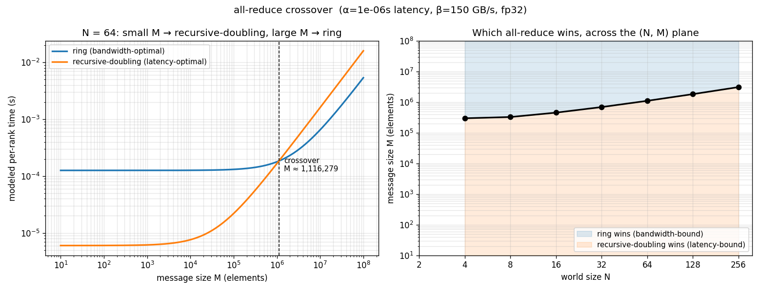
Small messages, many ranks → latency dominates → recursive-doubling. Large
messages → bandwidth dominates → ring. The boundary moves with the fabric:
faster links (bigger β⁻¹) push it one way, higher latency α the other.
Why this matters in Megatron
This is not academic. In a single Megatron-LM training job, two different all-reduces live on opposite sides of that crossover line:
- Tensor-parallel (TP) does an all-reduce inside every layer, on the critical path of forward and backward — small-to-medium messages, exquisitely latency-sensitive. That is why TP is kept inside a node, on NVLink, and why it wants the latency-optimal regime.
- Data-parallel (DP) does one big gradient all-reduce per step, off the critical path and overlappable with backward — large messages, bandwidth-bound, spanning nodes. That is the ring regime.
Same contract, same all_reduce call in your code. Different algorithm
underneath, because (N, M, latency-vs-bandwidth) lands them in different parts
of the plane. The library morphs the realization for you — and now you can
see exactly the surface it is morphing across.
Code, the measurement harness, and the plotting script:
neural-nets/projects/01-collectives.
Next in the track: relaxing the contract itself.