Physics-Informed Neural Networks for Plasma: A Challenger to the Mesh

Status — work in progress (2026-06-14). Phase 1, the framework, is complete: a from-scratch PINN stack solving six progressively harder plasma PDEs, each validated against an analytical or manufactured reference (results below). Phase 2, the benchmark, has results on three problem classes: the matched-accuracy wall-clock head-to-head is done on 1-D diffusion (~40,500×), coupled tokamak transport (~49,800×), and Grad-Shafranov equilibrium (~37,400×) — the classical solver wins every one. The training loop is profiled too — on Apple MPS and an NVIDIA H100 (the H100 gives ~6× and makes float64 free, but the loop stays launch-bound). A high-dimensional crossover hunt found no crossover on smooth Poisson (the gap widens, the PINN breaks by d=5). Inverse-problem results are in — and they completed the honest arc. A scalar unknown favours classical. Recovering an ill-posed field D(x) looked like the PINN's niche — it beat a naive (unregularized) classical baseline 14.5% vs 35–90%. But once the classical inversion is given the same smoothness prior (first-order Tikhonov, λ chosen blind), it wins: ~11% L2, K-robust, and ~10²–10³× faster. The PINN's apparent edge was an artifact of an unregularized opponent. Across every head-to-head tried, the regularized mesh method wins; the prior, not the network, is what tames the inverse problem.

The challenge

The PENNANT methodology campaign represents the established paradigm: discretize the domain into a mesh, march the governing equations forward, and pour engineering effort into making the irregular memory access go fast on a GPU. It works, it is trusted, and it is hard.

Physics-informed neural networks (PINNs) propose a different bargain. Instead of a mesh, represent the solution field as a neural network and train it so that the governing PDE residual — the physics itself — is the loss function. No discretization, mesh-free, naturally differentiable, and a representation that maps cleanly onto the dense tensor math GPUs are actually built for.

The scientific-ML literature is full of demonstrations that PINNs can solve a given PDE. It is much quieter on the question a performance engineer has to ask:

At a fixed target accuracy, does the PINN reach the answer in less wall-clock time than a well-implemented classical solver — and if so, on which problems?

This campaign sets out to map that boundary honestly, on plasma problems specifically, because plasma is where the personal stake is: the work points toward fusion simulation, where the governing systems are stiff, multiscale, and brutally expensive for classical methods.

But before you can benchmark a method, you need a correct, trusted implementation of it. That is Phase 1.

Phase 1 — a validated PINN framework (complete)

Rather than a single demo, the framework is a staircase: each phase adds exactly one new difficulty, and nothing advances until it is validated against a reference. Pure PyTorch, no PINN wrapper libraries — every component visible and understood.

Phase	Problem	New difficulty	L2 vs. reference
1a	1-D slab diffusion	baseline	6.4e-4
1b	coupled density + temperature	nonlinear coupling	n 2.7e-5 · T 2.0e-5
2a	Grad-Shafranov equilibrium	2-D elliptic, 1/r singularity	1.1e-4
2b	cylindrical transport	curved geometry	4.6e-5
3	tokamak flux-surface transport	coupling and geometry	n 6.7e-5 · T 4.8e-5
4	self-consistent equilibrium + transport	two-way feedback	n 7e-6 · T 3e-6 · g 1.7e-6

Two ideas carried every phase: hard constraints (boundary/initial conditions baked into the network architecture, so they hold exactly and the optimizer has a single objective — the physics) and manufactured solutions (choose an exact answer, derive the source term that makes it true, validate against it — the source algebra verified to machine precision before any long run).

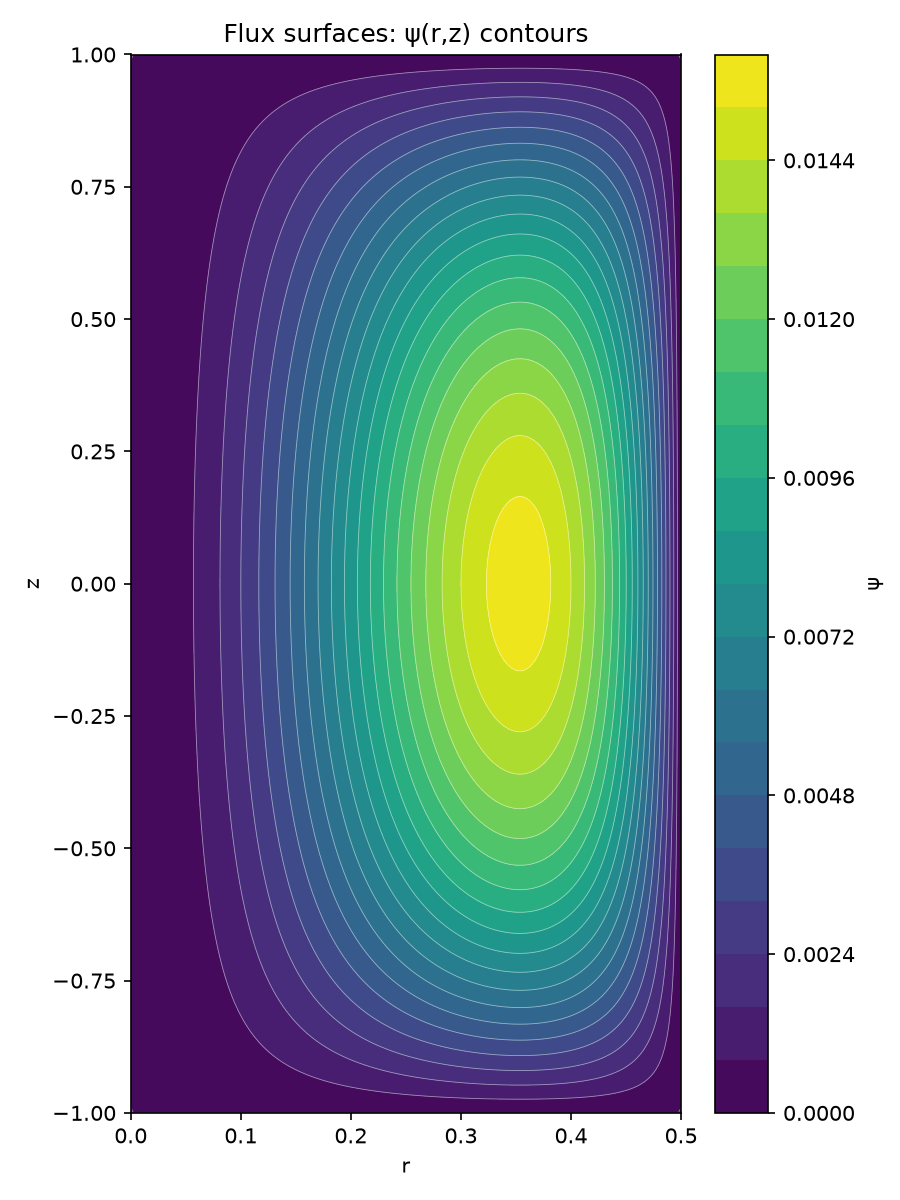
The equilibrium and its flux surfaces

The Grad-Shafranov equation gives the magnetic flux function whose contours are the surfaces that confine the plasma. The 1/r axis singularity is removed analytically; all boundary conditions are structural.

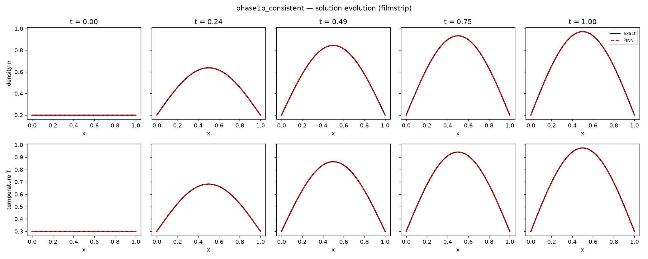
Transport that evolves in time

Coupled density and temperature on a tokamak flux coordinate — the 1.5-D model real fusion codes use. PINN (red) against the manufactured exact solution (black), swept through time:

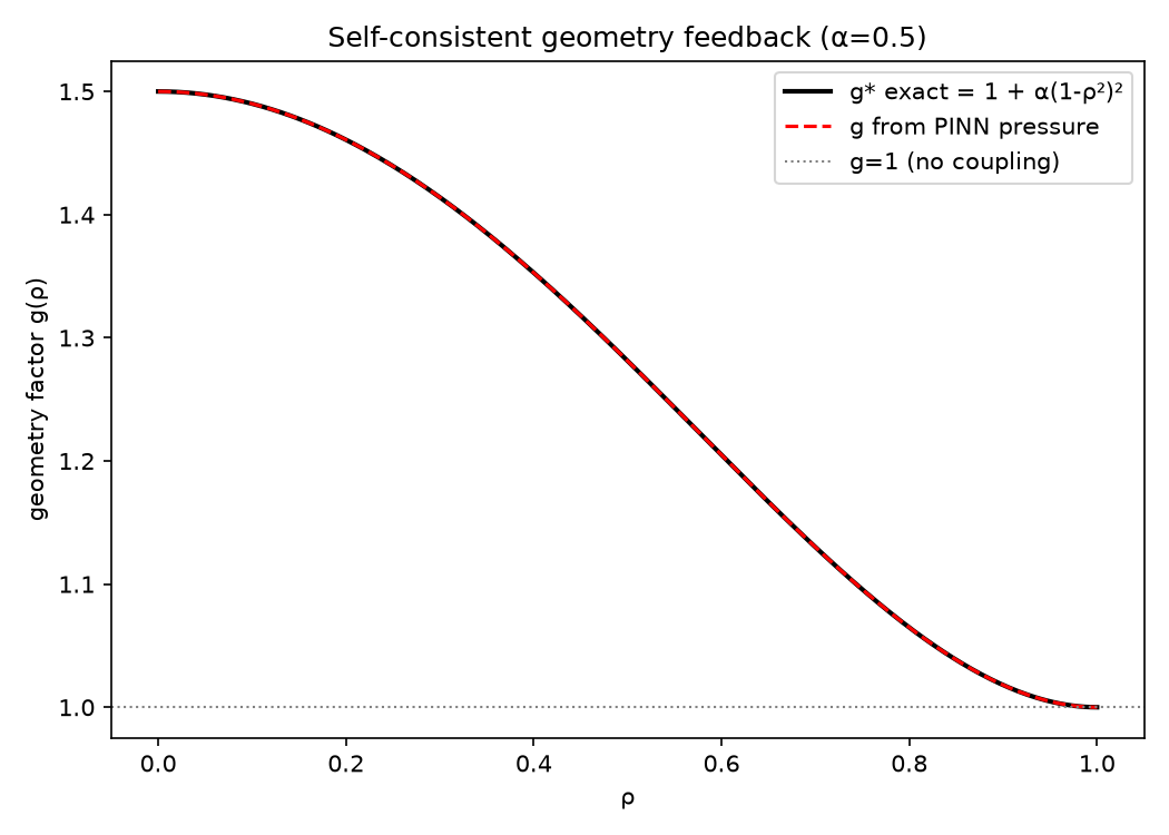
The capstone: self-consistency

In a real plasma, pressure sets the magnetic geometry and the geometry feeds back into transport. Phase 4 solves both in one network, with the geometry computed from the network's own pressure inside the loss. The proof it is truly self-consistent: the geometry implied by the converged solution matches the geometry that produced it to one part in a million.

The most useful result was a failure

Phase 1b first failed on temperature — 20% error — and the diagnosis is the part worth keeping. Temperature is energy per particle, T = (nT)/n; wherever the density goes to zero (at t=0 and at the walls) it is mathematically ill-defined, and the reference solver's recovery of it is noise. The fix was not more compute but a well-posed formulation: a density floor so the field is defined everywhere, a consistent initial condition, and validation against a direct manufactured temperature. Error fell from 20% to 0.002% — about ten-thousand-fold.

That episode is the whole ethos of this campaign in miniature: diagnose honestly, fix the formulation, measure the result.

Walkthrough deck: an interactive slide deck (offline, self-contained) covers the method, what a PINN model actually is at the matrix level, and every phase with figures and animations.

What is a PINN, really? A companion visual explainer (offline, self-contained) walks the method in seven acts — the canonical equations and the network diagram, a convergence proof that unregularized PINNs overfit catastrophically (Doumèche, Biau & Boyer 2026), the head-to-head against a mesh, and a plain ledger of what a PINN is and is not. Built to teach the method honestly, priors and failure modes included.

Why plasma, and why this matters for fusion

Plasma systems are attractive PINN targets and adversarial ones: stiff transport, disparate timescales, sharp gradients at boundary layers. The phases above deliberately march toward the structure of real reduced fusion models — flux-surface transport coupled to MHD equilibrium — because that coupling is where classical methods get expensive and where a mesh-free, differentiable representation might eventually earn its place.

The honest framing: classical solvers are extraordinarily good at these problems. A PINN does not win by default. The campaign is a search for the regime — high dimension, parametric sweeps, inverse problems, self-consistent coupling — where the mesh-free representation finally pays for itself.

The benchmark — first result (Phase 2)

The methodology, mirroring the profiling methodology post: fix one accuracy target per PDE and measure time to reach it for both methods; keep the classical baseline competent (not a strawman); and map where the crossover lives. The first problem — 1-D diffusion — is done, on the same machine (CPU). The classical baseline is a Crank-Nicolson finite-difference solver (sparse tridiagonal solve, verified 2nd-order convergent); the PINN is the hard-constraint architecture from Phase 1, float64, early-stopped at the target.

Where the classical solver still wins — measured

Single instance, matched accuracy (target L2 = 1e-3):

Method	Time to L2 = 1e-3
Classical (Crank-Nicolson, nx=61)	0.78 ms
PINN (hard-constraint, float64)	31.7 s

The classical solver is ~40,500× faster to the same accuracy.

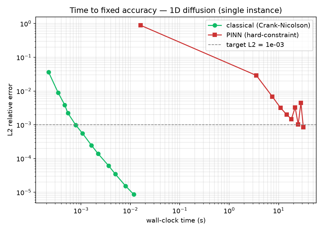
For a smooth, low-dimensional, single-instance PDE this is exactly what theory predicts, and it is the result that earns the reader's trust: the mesh is extraordinarily efficient, and the PINN pays a large fixed training cost. No amount of framing changes it.

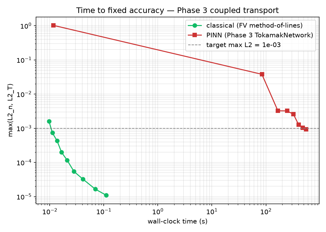
The same holds for a coupled, nonlinear system. Repeating the test on Phase 3 — tokamak flux-surface transport of density and temperature together, the 1.5-D model real fusion codes use — against a competent finite-volume method-of-lines solver:

Method	Time to max(L2ₙ, L2_T) = 1e-3
Classical (FV method-of-lines)	11 ms (M = 30 grid)
PINN (coupled two-field)	555 s (3500 Adam steps)

→ ~49,800× in the classical solver's favour — a slightly wider gap than the 1-D case, because the two-field PINN costs more to train while the coupled solver stays in milliseconds. The 1/ρ geometry and the n–T nonlinearity do not move the boundary at single-instance, low dimension.

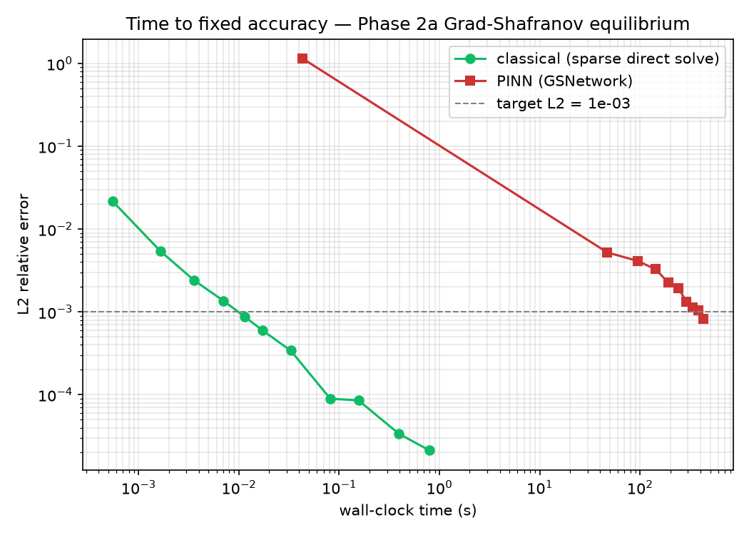
And for an elliptic equilibrium. The third problem, Grad-Shafranov (Phase 2a), is a boundary-value problem with no time — the competent classical method is a single sparse direct linear solve, not time-stepping:

Method	Time to L2 = 1e-3
Classical (sparse direct solve)	11 ms (nr = 51 grid)
PINN (GSNetwork)	428 s (4500 Adam steps)

→ ~37,400×. Three problem classes now — scalar parabolic, coupled nonlinear transport, and elliptic equilibrium — and the classical solver wins every one by 37,000–50,000×. The verdict does not depend on the kind of PDE.

Where the PINN starts to pay off — not here, and the data says so

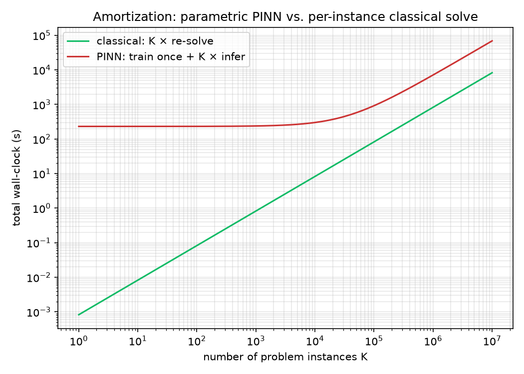
The PINN's structural argument is amortization: train once over a family of problems, then answer any member by inference, while the classical solver re-solves from scratch each time. Tested on 1-D diffusion with the source location as a free parameter x0 ∈ [0.3, 0.7]:

Quantity	Value
PINN train once (mean L2 = 3e-3)	232 s
PINN inference per instance	3.9 ms (single) · 6.9 ms (batched, CPU)
Classical solve per instance	0.83 ms

The PINN never breaks even on this problem. Its per-instance inference alone (3.9 ms) already exceeds a full classical solve (0.83 ms), so amortizing the training cost is moot. Even granting free inference, break-even would require ≈ 280,000 instances.

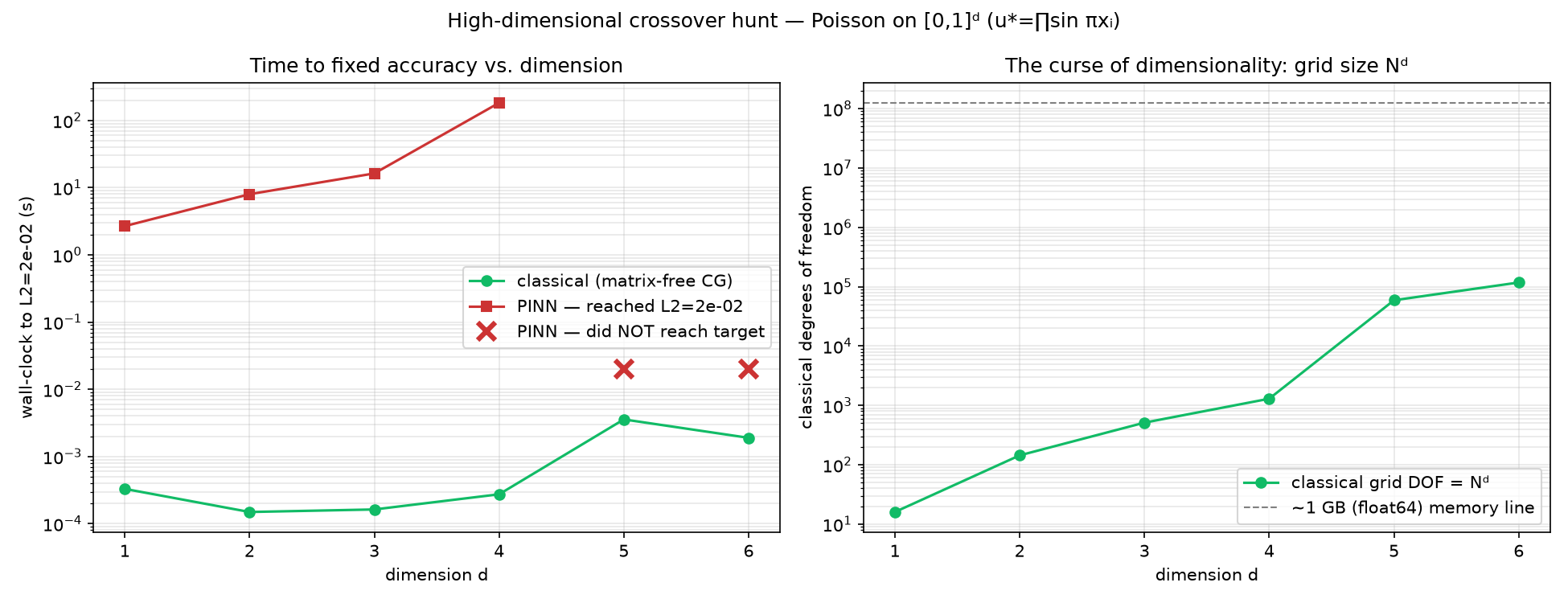
So where does the mesh-free representation pay off? The strongest theoretical case is high dimension — a tensor grid has Nᵈ nodes, so the mesh should eventually become infeasible. We went looking for that crossover on the d-dimensional Poisson problem, d = 1 → 6:

d	classical	PINN
1	0.3 ms	2.7 s
3	0.2 ms	16 s
4	0.3 ms	182 s
5–6	< 4 ms	could not reach 2% (best L2 0.43, 0.85)

The crossover did not appear — the gap widened, then the PINN broke. Honestly, the opposite of the hoped-for result, for an instructive reason: a smooth solution needs only a coarse grid, so Nᵈ stays tiny (a few thousand nodes even at d=6) and the mesh never pays the curse — while the PINN pays a different curse, as Monte-Carlo collocation of the cube gets exponentially sparser and the optimisation gets harder, until it can't hit 2% at all by d=5.

So a PINN does not get a free high-dimensional win. The regime where the mesh-free representation genuinely earns its place is narrower than the hype: problems where the grid is forced to be enormous or cannot be built at all (unrepresentable 5–6-D kinetic/gyrokinetic distributions), or where standing up and regularizing the classical machinery is itself the hard part. The obvious candidate — inverse / data-assimilation problems — we expected to be the PINN's home turf; the next section tests that and finds even there a fairly regularized classical solver wins.

The PINN's predicted niche — inverse problems — and how it dissolved under a fair test

So we tested that prediction: infer an unknown diffusivity from sparse, noisy measurements of the solution — what fusion transport analysis actually does (recover D, χ from measured profiles).

A scalar unknown still favours the classical method — least_squares around a forward solver recovers it ~3,000× faster and far more robustly (the scalar PINN collapses to 97% error at 10% noise). One unknown is not the niche.

Recovering a spatially-varying field D(x) looked like the flip. Against a naive classical baseline — nodal least-squares with no regularization — the PINN was the most accurate, and the classical inversion got worse as the number of unknowns grew (35% → 56% → 90% error): with 15 nodes the recovered D(x) oscillates wildly, the textbook signature of an ill-posed inverse problem overfitting noise. Tempting to call it the genuine PINN niche.

But that comparison was rigged: the PINN had a smoothness prior and the classical baseline had none. So we built the fair competitor — give the classical inversion the same prior the PINN carries (first-order Tikhonov, penalising ∫(dD/dx)², with λ chosen blind by the discrepancy principle):

method	D(x) error	cost (single fit)
PINN (one run)	14.5%	189 s
Tikhonov classical, 5 nodes	10.8%	0.10 s
Tikhonov classical, 9 nodes	11.5%	0.16 s
Tikhonov classical, 15 nodes	11.5%	0.26 s
naive classical (no prior)	35–90%	—

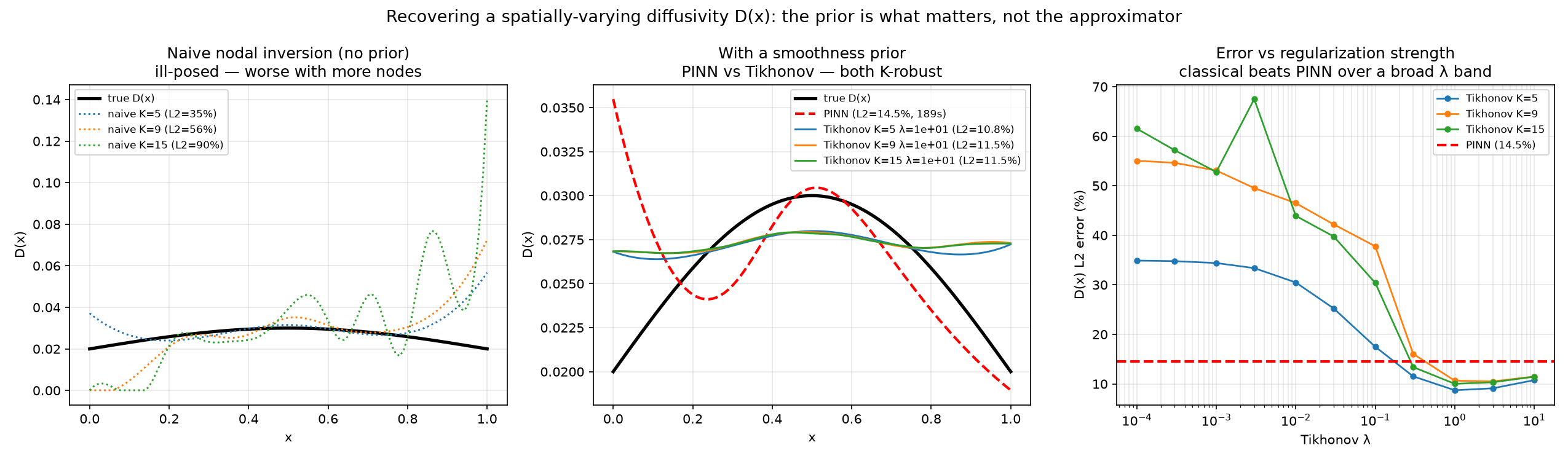
Once the classical inversion carries a matched prior, the PINN's advantage disappears. The regularized mesh method is more accurate (~11%, or ~9% at the oracle λ, vs the PINN's 14.5%), it is K-robust (the error stops growing with the number of nodes), and it is ~10²–10³× faster — a single fit is under a second; even the whole λ-selection sweep is a few seconds against 189 s for one PINN training run. The result holds over a broad band of λ (right panel).

The PINN's apparent win was an artifact of comparing against an unregularized opponent. The deeper lesson is the opposite of the hype, and it is the same lesson a recent production stellarator-optimization paper reaches independently (Landreman et al. 2026, which uses no neural surrogate): in an ill-posed inverse, the prior is what tames the problem, not the function approximator — and once you have the prior, the cheapest vehicle for it (a mesh, a Gaussian process) wins. The PINN's real value is feasibility — standing up a differentiable, mesh-free solver where building and regularizing the classical machinery is itself the hard part — not raw accuracy or speed.

Is the PINN training loop actually GPU-friendly? — measured (Apple M4 / MPS)

The training step was profiled on the available hardware — an Apple M4 with the MPS (Metal) backend; no NVIDIA, so this is not CUDA/Nsight. The answer is the one practitioners rarely hear: at this scale, the GPU barely helps, and the precision the physics needs rules it out anyway.

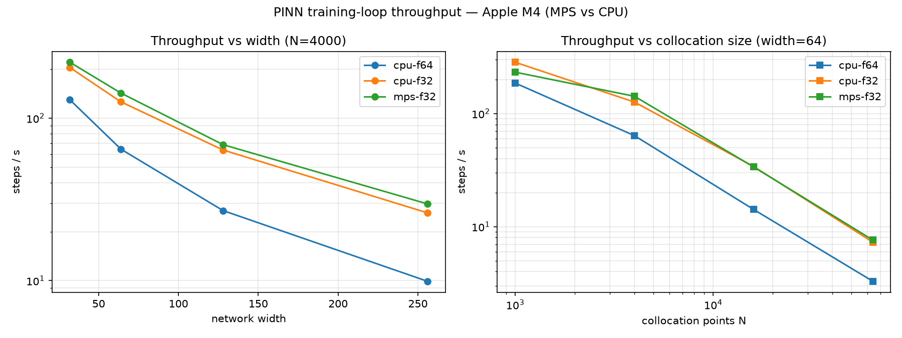
• The loop is autograd-bound, not compute-bound. The forward derivative graph (autograd assembling ∂u/∂x and ∂²u/∂x²) plus the double-backward are ~98% of each step; the optimizer is ~1.5%. The op profile shows the cause — thousands of tiny ops from the nested-derivative graph (1,340 matrix-multiply and 380 double-tanh-backward calls per 20 steps), dominated by many small mm, mul, and tanh_backward.
• The GPU gives ~1.13× over CPU at the same precision — and at some problem sizes the CPU is actually faster. The small ops never saturate the GPU; launch and dispatch overhead dominate.
• float64 costs ~2× on CPU and cannot run on MPS at all. The nonlinear plasma physics needs float64, so the accurate lane is locked to the CPU — the GPU is doubly unhelpful.

This is the performance-engineering result a pure-ML write-up would miss: a PINN is assumed to be GPU-friendly because it is "just" tensor math, but its defining feature — differentiating the network to form the PDE residual — generates an autograd graph of many small operations that a GPU executes inefficiently.

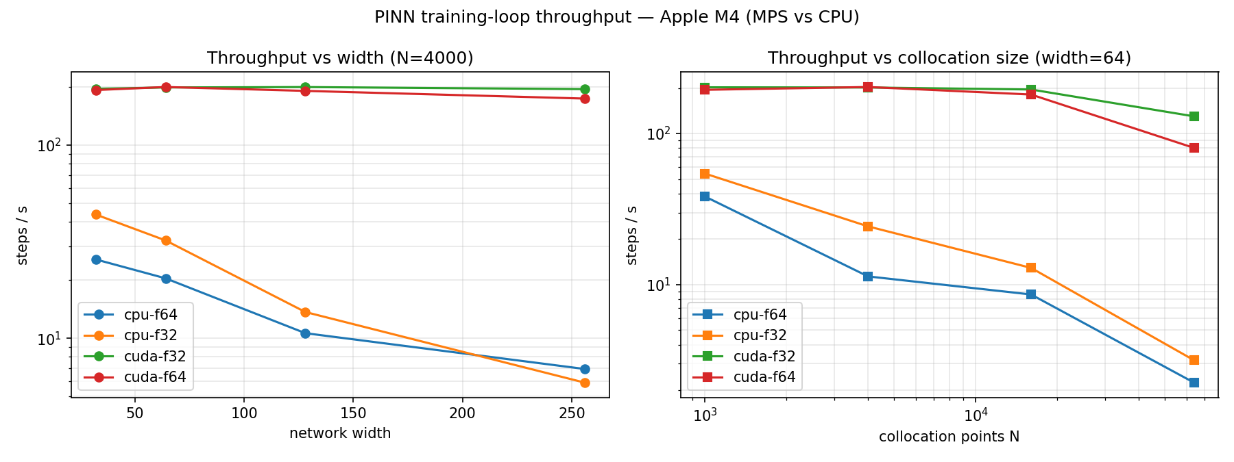
Cross-checked on an NVIDIA H100 (cloud, via Brev — torch 2.6 / CUDA 12.4, Nsight Systems). A real data-center GPU does help — but the launch-bound ceiling holds:

	Apple M4 (MPS)	NVIDIA H100
GPU vs same-box CPU (f32)	~1.1×	6.0×
float64 penalty	impossible on MPS	~free (cuda-f64 ≈ cuda-f32)
throughput vs width / N	flat	flat (~190 steps/s)

Three measured results: (1) the H100 gives a real but modest 6× — not 100× — because the loop is overhead-bound; (2) float64 is essentially free on the H100 (versus a ~2× CPU tax and no float64 on MPS), which matters for precision-hungry scientific PINNs; (3) it is still launch-bound — Nsight shows cudaLaunchKernel is 83 % of CUDA API time (81,504 launches over 200 steps), the nested-derivative graph dissolving into tens of thousands of ~2 µs kernels. Even an H100 spends most of its host time launching, not computing — and a 6× speedup leaves the PINN ~4 orders of magnitude behind the classical solver on forward solves.

Why it matters for clients

Scientific ML is being adopted faster than it is being honestly benchmarked. Organizations investing in surrogate models, PINNs, and neural operators need to know not whether the method can work in a demo, but whether it beats their existing solver on their problem, at their accuracy bar, on their hardware — and where it doesn't.

This campaign is a template for that evaluation: a correct, validated implementation first (Phase 1, done), then a matched-accuracy comparison against an honest baseline (Phase 2, first result in — and it says use the mesh for this class of problem). It separates the problems where neural methods are a genuine win from the ones where a well-tuned classical solver is still the right answer — and so far, on smooth low-dimensional PDEs, the classical solver is the right answer by a wide margin.

The full framework code, per-phase data, validation figures, and the walkthrough deck are linked below.

References

• R. D. Hazeltine and J. D. Meiss, Plasma Confinement. Dover Publications, 2003 (orig. Addison-Wesley, 1992). — equilibrium concepts: MHD force balance, flux surfaces, and the Grad-Shafranov equation behind the equilibrium phases.
• T. E. Evans, "Implications of Topological Complexity and Hamiltonian Chaos in the Edge Magnetic Field of Toroidal Fusion Plasmas," in Chaos, Complexity and Transport: Theory and Applications (eds. C. Chandre, X. Leoncini, G. M. Zaslavsky), World Scientific, 2008, pp. 147–176. — chaotic edge transport (ELMs, stochastic field lines) and the Hamiltonian field-line picture: why fusion transport is a hard, multiscale target.
• F. L. Hinton and R. D. Hazeltine, "Theory of plasma transport in toroidal confinement systems," Rev. Mod. Phys. 48, 239 (1976). — the flux-surface-averaged transport theory behind the Phase 3 equations.