Plasma-PINN

Physics-Informed Neural Networks
for Fusion Plasma PDEs

Progressive framework: 1D diffusion → self-consistent tokamak equilibrium + transport
Pure PyTorch · validated at every stage

Srinath Vadlamani · SV Advanced Computing LLC

The goal

Solve fusion-plasma PDEs from first principles — no PINN wrapper libraries
Build complexity in stages; validate each against analytical / manufactured solutions
Every component visible and understood
End state: self-consistent equilibrium + transport

Phase 1a  1D diffusion        ✓
Phase 1b  coupled n,T         ✓*
Phase 2a  Grad-Shafranov      ✓
Phase 2b  cylindrical n       ✓
Phase 3   tokamak n,T         ✓
Phase 4   self-consistent     ✓

The PINN method

Approximate the PDE solution with a network u_θ(x,t). PyTorch autograd gives exact derivatives, so the PDE residual becomes a loss term — no mesh, no discretization.

tanh activation — infinitely differentiable
float64 on CPU — precision for nonlinear terms
Adam → L-BFGS — explore, then polish

L = w_pde·‖R(x,t)‖²
  + w_bc ·‖u-g‖²
  + w_ic ·‖u-f‖²

R = ∂ₜu - D∂ₓₓu - S

Two ideas that made it work

Hard constraints

Bake BCs/ICs into the network output so they hold exactly — zero BC/IC loss, optimizer has one objective.

ψ = r²(R²-r²)(Z²-z²)·NN
n = t(1-ρ²)·NN

Manufactured solutions

Pick an exact solution, derive its source analytically, train against it. Exact reference, no solver.

verified: residual
→ 1e-16 (machine zero)

What is truly being modeled?

The network is the solution field itself — a continuous, infinitely-differentiable surrogate u_θ(x,t) for n, T, ψ …

Not a discretization — no mesh, no time-stepping
Not curve-fitting data — there is no dataset
We fit a function whose derivatives obey the conservation laws
The "training set" = collocation points where we demand the physics hold

u_θ : (x,t) ↦ field

physics IS the loss:
  R[u_θ] = 0   everywhere

θ chosen so the surrogate
satisfies the PDE,
not so it matches samples

The terms — coupled transport

  ∂n/∂t   =   D ∂²n/∂x²        +  S_n
  ─────       ──────────          ───
  density     particle           fueling /
  evolves     diffusion          ionization

  (3/2) ∂(nT)/∂t  =  χ ∂/∂x(n ∂T/∂x)  +  S_E
  ──────────────     ───────────────     ───
  thermal energy     conductive heat      heating
  (3/2 nT) rate      flux divergence      power
                     (χ = diffusivity,
                      n weights the flux)

Nonlinearity lives in n·T and n·∂ₓT — the energy equation couples to density. Geometry (Phase 2b/3/4) adds a 1/r or 1/ρ factor from the divergence in curved coordinates.

The wiring

  (x, t)                      inputs (collocation point)
    │
    ▼
  envelope · MLP_θ            hard constraint × network
    │                           e.g. n = n_e + x(1-x)t · NN
    ▼
  n(x,t),  T(x,t)            continuous fields  ◄─ the model
    │
    ▼  torch.autograd (exact derivatives)
  ∂ₜn  ∂ₓₓn   ∂ₜ(nT)  ∂ₓT  ∂ₓₓT
    │           [ + g(n,T) self-consistent geometry, Ph.4 ]
    ▼  assemble PDE residual
  R_n = ∂ₜn − D∂ₓₓn − S_n      R_E = 3/2 ∂ₜ(nT) − χ∂ₓ(n∂ₓT) − S_E
    │
    ▼
  L = ‖R_n‖² + ‖R_E‖²   ──►  Adam → L-BFGS  ──►  update θ
    └──────────────────  repeat until  R → 0  ──────────────┘

The network, as matrices

  z⁰ = [x, t]ᵀ                         ∈ ℝ²     inputs (coordinates)
  z¹ = tanh(W¹ z⁰ + b¹)                ∈ ℝ¹²⁸   W¹ ∈ ℝ¹²⁸ˣ²
  z² = tanh(W² z¹ + b²)                ∈ ℝ¹²⁸   W² ∈ ℝ¹²⁸ˣ¹²⁸
        ⋮     6 hidden layers, width 128         (tanh each)
  z⁶ = tanh(W⁶ z⁵ + b⁶)                ∈ ℝ¹²⁸
  u  = W⁷ z⁶ + b⁷                      ∈ ℝ²     W⁷ ∈ ℝ²ˣ¹²⁸  → (n,T)

  every layer = an AFFINE map  (Wz + b)  followed by a bend (tanh)

Dimension flow

 2 → 128 → 128 → 128
   → 128 → 128 → 128 → 2
(x,t)   features      (n,T)

Where the 83k numbers live

W¹: 128·2 +128 =    384
W²…W⁶: 5·(128²+128)=82 560
W⁷:   2·128 +  2 =    258
────────────────────────
θ total          ≈ 83 202

The model is these weights θ. Training shapes one continuous function ℝ²→ℝ² so it obeys the PDE.

What one layer actually does

one hidden unit j:
  hⱼ = tanh( Σᵢ Wⱼᵢ zᵢ + bⱼ )
      └ a soft step / bend,
        oriented by row Wⱼ,
        shifted by bⱼ

a layer = 128 bends in parallel
depth   = bends composed on bends
        → arbitrarily curved
          surfaces

Why the nonlinearity is essential

drop tanh ⇒ identity:
  u = W⁷ W⁶ … W¹ z
    = (one matrix) · z
  → only a flat plane

tanh is what lets the
stack BEND into a
PDE solution

tanh also has smooth derivatives of all orders — required to form ∂ₓₓu.

A model is a family of functions

  polynomial   u(x) = Σ cₖ xᵏ                 basis fixed (monomials)
  Fourier      u(x) = Σ cₖ sin(kπx)           basis fixed (sines)
  finite elem. u(x) = Σ cₖ φₖ(x)              basis fixed (hat fns)
  ───────────────────────────────────────────────────────────────
  neural net   u(x) = W⁷ tanh(… tanh(W¹x))    basis LEARNED & nonlinear

Classical methods fix a basis and solve a linear system for the coefficients c. A neural net lets the basis itself adapt — the weights reshape the building blocks and their amplitudes together.

Same idea as spectral/FEM solvers: represent u in a basis
Difference: the basis is nonlinear, high-dimensional, and learned
Cost: the fit is a nonconvex optimisation (Adam → L-BFGS)
Payoff: mesh-free, smooth, same recipe in 1D, 2D, coupled, nonlinear

A tiny worked example (2 → 3 → 1)

input  z = [x, t]ᵀ

        ⎡ 0.5  -0.3⎤              ⎡ 0.5x - 0.3t⎤
  W¹ =  ⎢ 0.1   0.8⎥   a = W¹z = ⎢ 0.1x + 0.8t⎥
        ⎣-0.6   0.2⎦              ⎣-0.6x + 0.2t⎦

  h = tanh(a) ∈ ℝ³        W² = [1.2  -0.7  0.4]
  u = W²h = 1.2·h₁ - 0.7·h₂ + 0.4·h₃          (scalar output)

  e.g. at (x,t)=(1,0):  a=[0.5,0.1,-0.6]ᵀ
       h=[0.462,0.100,-0.537]ᵀ   u = 0.270

u is an explicit closed-form expression in (x,t). The real network is this exact structure — just 128 wide and 6 deep.

Derivatives are matrices too

chain rule through the toy net  (tanh' = 1-h²,  tanh'' = -2h(1-h²)):

  ∂u/∂x   = W² · [ (1-h²) ⊙ W¹₍:,1₎ ]
  ∂²u/∂x² = W² · [ -2h ⊙ (1-h²) ⊙ W¹₍:,1₎² ]
                              ( W¹₍:,1₎ = first column = ∂a/∂x )

assemble the physics residual (1D diffusion):
  R(x,t) = ∂ₜu  −  D ∂ₓₓu  −  S(x)

loss over N collocation points, minimise over the weights:
  L(θ) = (1/N) Σᵢ R(xᵢ,tᵢ)²        θ* = argmin_θ L(θ)

autograd evaluates exactly these expressions — we never derive them by hand. The residual is a closed-form function of θ.

Results at a glance

Phase	Problem	L2 error	Status
1a	1D slab diffusion	6.4e-4	✅ PASS
1b	Coupled n,T (consistent-IC fix)	n 2.7e-5 / T 2.0e-5	✅ PASS
2a	Grad-Shafranov equilibrium	1.1e-4	✅ PASS
2b	Cylindrical transport	4.6e-5	✅ PASS
3	Tokamak coupled n,T	n 6.7e-5 / T 4.8e-5	✅ PASS
4	Self-consistent eq+transport	n 7e-6 / T 3e-6 / g 2e-6	✅ PASS

L2 relative error vs analytical / manufactured reference

Phase 1a — 1D diffusion

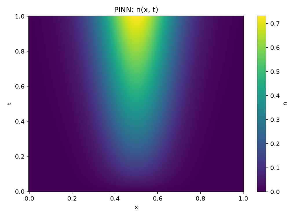
∂n/∂t = D ∂²n/∂x² + S(x)

The clean baseline: single linear field
MLP 4×64, Adam on MPS GPU
L2 = 6.4e-4 vs Fourier-series exact

Density builds from zero to the steady parabolic profile balancing source against wall losses.

Phase 1b — the instructive failure

  ∂n/∂t        = D ∂²n/∂x² + S_n
  (3/2)∂(nT)/∂t = χ ∂ₓ(n ∂ₓT) + S_E

  result:  n  0.9%   PASS
           T  19.6%  FAIL

Density passed; temperature failed badly
Root cause: T = (nT)/n is ill-defined where n→0 — that's everywhere at t=0 and at the walls
The FD reference's T = p/(n+ε) is noise there; no well-defined truth to match

(An earlier note blamed a T_init corner conflict — the config showed T_init=0; the real cause is the degeneracy.)

Phase 1b — the fix works

n,T(x,t) — PINN (red) vs exact (black)

Make it well-posed:

density / T floor → n,T > 0 everywhere
consistent IC = BC = edge value
hard constraint n = n_e + x(1-x)t·NN
direct-field MMS — never compute p/n

T:  19.6%  →  0.002%
        (≈ 10⁴× better)
n 2.7e-5   T 2.0e-5  PASS

Phase 2a — Grad-Shafranov equilibrium

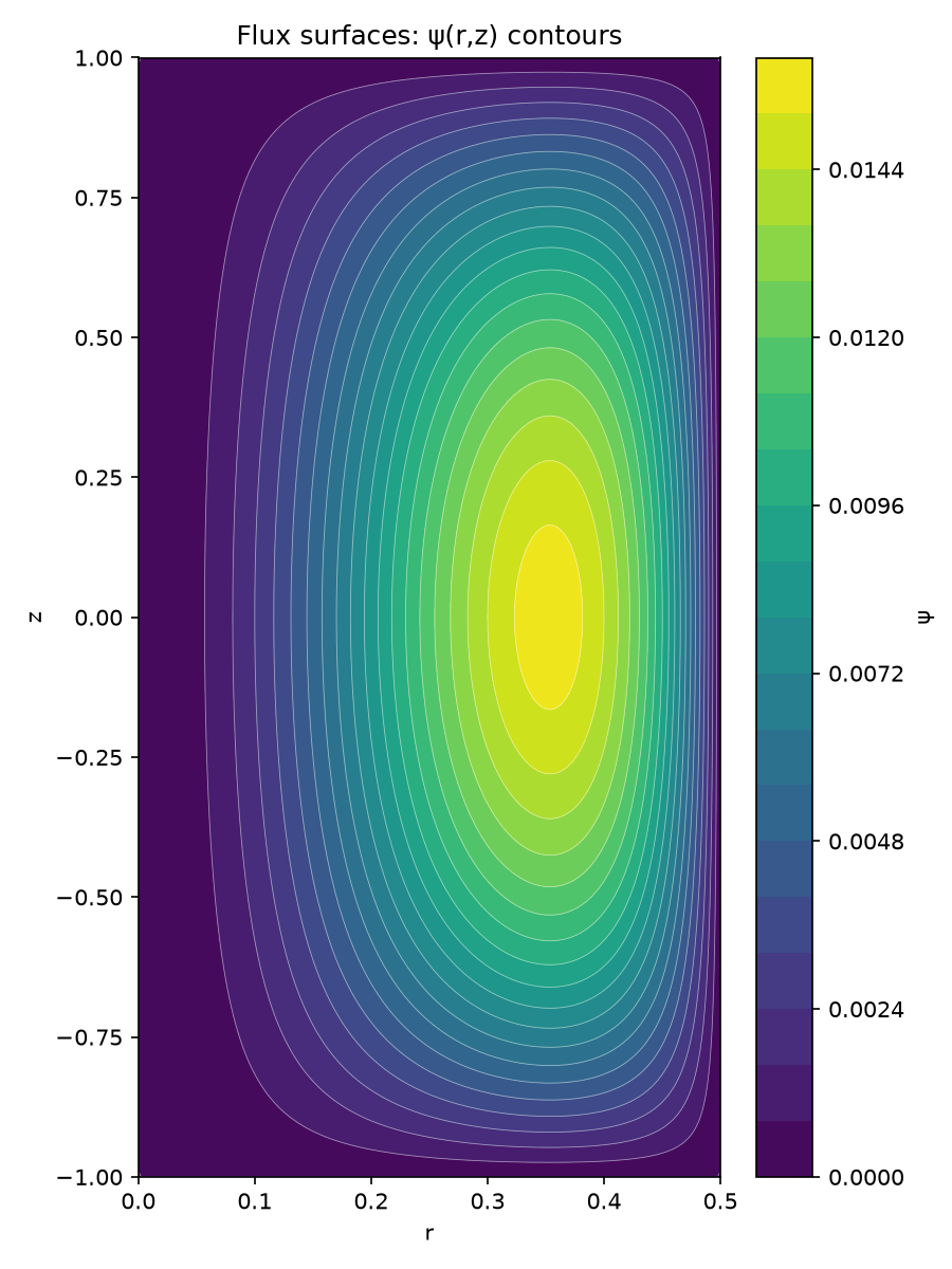
ψ_rr − (1/r)ψ_r + ψ_zz = F

2D elliptic MHD equilibrium; flux surfaces = contours of ψ
1/r singularity removed by ×r regularisation
Hard constraint enforces all BCs + axis regularity
L2 = 1.1e-4 — EXCELLENT by step 2000

Phase 2b — cylindrical transport

n(r,t) — PINN (red) vs exact (black)

∂n/∂t = D(∂²n/∂r² + (1/r)∂n/∂r) + S

Geometry factor before coupling
Hard constraint t(R²−r²)·NN(r²,t)
L2 = 4.6e-5

Parabolic profile builds to steady state as the source fills the column.

Phase 3 — tokamak coupled transport

n,T(ρ,t) — PINN (red) vs exact (black)

1.5D flux-surface transport (ASTRA/TRANSP model)

Combines coupling + 1/ρ geometry + many BCs
Same coupled n,T that failed in 1b → now n 6.7e-5, T 4.8e-5
4000× better on T — architectural, not more training

Phase 4 — self-consistent equilibrium + transport

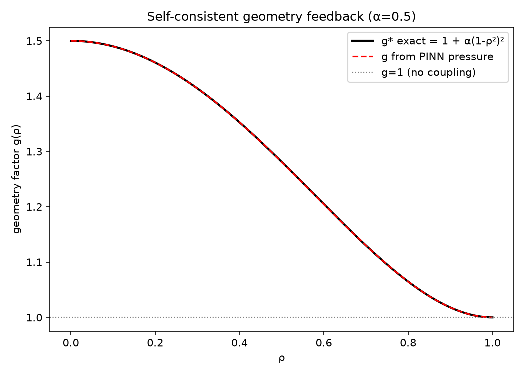
Pressure from transport sets the geometry; geometry feeds back into transport. Solved together:

g(ρ) = 1 + α·p(ρ)/p(0)
  (computed inside the loss)

The self-consistency proof

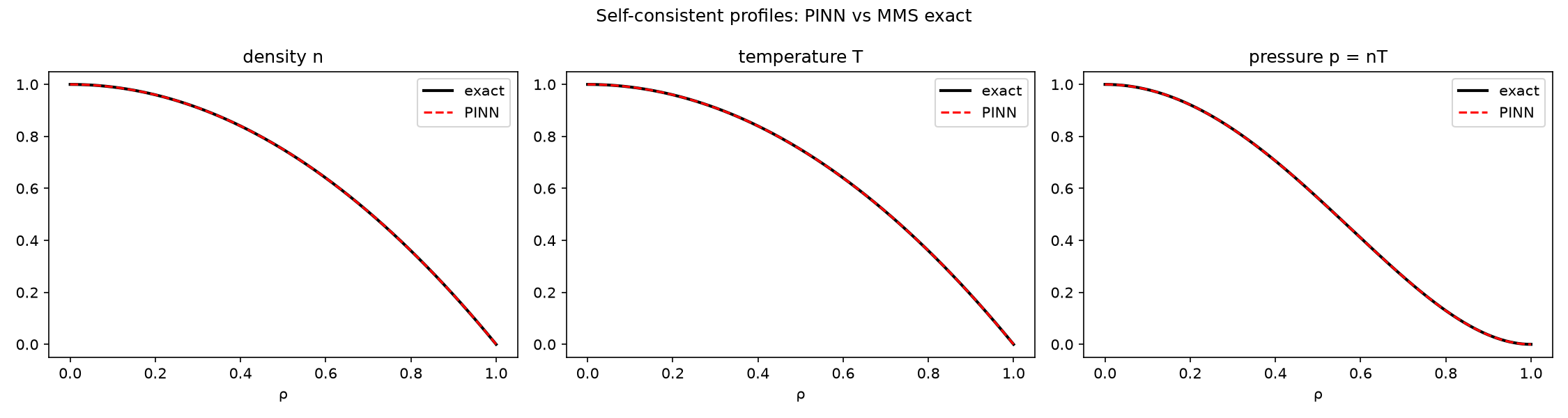
n = 7.1e-6, T = 2.9e-6
g = 1.7e-6 — the geometry implied by the solution matches the geometry that produced it

Equilibrium and transport are mutually consistent — the fixed point was found.

How training converges

L2 quality labels
──────────────────────────
>50%    untrained
20-50%  coarse shape
5-20%   structure emerging
2-5%    near target
0.5-2%  PASS
<0.5%   EXCELLENT

Mid-training callbacks report true L2 vs reference, not just loss
Hard-constraint phases hit EXCELLENT by step 2000
L-BFGS often flat — Adam already at machine precision
Loss spans up to 14 orders of magnitude (Phase 4)

What carried through

Architecture > iterations

Bake every enforceable constraint into the network; leave the optimizer one objective.

MMS everywhere

Manufactured solutions give exact references with verified sources — no solver noise.

Precision matters

float64 + CPU L-BFGS; MPS float32 silently stalls on nonlinear PDEs.

Well-posedness

Phase 1b: define what you can measure (avoid p/n where n→0).

From diffusion to self-consistency

Five phases, one recipe: hard constraints + manufactured solutions + Adam→L-BFGS in float64.

1a  6.4e-4   2a  1.1e-4   2b  4.6e-5
3   6.7e-5   4   7e-6  (+ g 1.7e-6 self-consistency)

Phase 4b — full 2D Grad-Shafranov geometry coupling
Physical sources & ASTRA/TRANSP benchmarking

codeberg.org/srinathv/plasma-pinn