Multigrid: The O(N) Idea, and What It Teaches a Loss Function

An algorithm with a ceiling you can prove

Most performance work is empirical. You measure, you tune, you measure again, and the honest answer to "how fast could this be?" is usually "faster than it is now, by an amount I will know when I get there." Multigrid is one of the few places where the mathematics hands you the answer in advance: for a well-posed elliptic problem with the right components, multigrid converges to a fixed tolerance in a number of iterations independent of the problem size, at O(N) total work. That is asymptotically optimal — you cannot beat reading the data once.

That is a strong claim, and the conditions on it matter. But the idea underneath is simple enough to state in a sentence, and it generalizes far beyond the PDE it was invented for. This post is what the idea is, where it argues with a GPU, and what it says about a loss function. Most of it is theory; one section is an experiment on rented hardware that contradicted my own model, and I have left the model in place so you can watch it fail.

The insight: error has a spectrum

Take a discretized elliptic PDE — a Poisson problem on a grid, say — and attack it with a simple iterative solver: Jacobi, or Gauss–Seidel. Watch the error.

For the first several sweeps it collapses. Then it stalls, and keeps stalling, and the iteration count you need to reach a tolerance grows as you refine the mesh. The solver has not stopped working. It has run out of the kind of error it is good at.

Decompose the error into the eigenmodes of the iteration matrix. A relaxation sweep damps the high-frequency, oscillatory modes strongly — those die in a handful of sweeps. It damps the low-frequency, smooth modes barely at all, and the smoother the mode, the less it does. Refine the mesh and you have simply introduced more smooth modes for it to fail on, which is exactly why the iteration count scales with N.

So a relaxation sweep is not really a solver. It is a smoother: a filter that removes oscillatory error and leaves smooth error behind. Naming it that way is the whole insight, because it turns "my solver stalled" into "my solver left behind a specific, characterized thing," and a characterized thing can be attacked on its own terms.

The move: make every mode oscillatory somewhere

Here is the observation that makes the method. A smooth error on a fine grid looks oscillatory on a coarse grid. Sample a slowly-varying function at half the points and, relative to the new grid spacing, it is no longer slowly varying. The error that the fine-grid smoother could not touch is precisely the error that a coarse-grid smoother can.

So you do this:

1. Smooth on the fine grid — a few relaxation sweeps kill the oscillatory error.
2. Restrict the remaining residual down to a coarser grid.
3. Solve the coarse-grid problem for a correction — recursively, because the once-smooth error is now oscillatory relative to the coarse grid, and whatever is still too smooth for that grid gets pushed down another level.
4. Prolong (interpolate) the correction back up to the fine grid and add it.
5. Smooth again, to clean up the high-frequency junk that interpolation introduced.

Recurse until the grid is small enough to solve exactly, and you have a V-cycle. Do more work on the way back up and you get a W-cycle; start on the coarsest grid and work up, and you get full multigrid (FMG).

Four components define the method: the smoother, the restriction operator R, the prolongation operator P, and the coarse-grid operator, usually taken as the Galerkin product R A P. Everything interesting about a particular multigrid method — and everything that can go wrong with it — lives in those four choices.

Why it is optimal

The reason multigrid attains O(N) is complementarity. The smoother and the coarse-grid correction each dispatch exactly the portion of the error spectrum that the other cannot see. Neither is a good solver. Together they leave the error nowhere to hide, and because the coarse levels are geometrically smaller, the total work in a cycle is a constant multiple of the fine-grid work — a convergent geometric series, not a multiplier that grows with N.

That is the whole argument, and it is worth internalizing because it is the template for a class of algorithms: find a basis in which your slow error is fast, and pay only a geometric tail for the privilege.

Algebraic multigrid (AMG) takes this seriously enough to drop the grid. Rather than coarsening geometry, AMG inspects the matrix — strength of connection between unknowns — and builds a coarse level and interpolation operator from the operator alone. That is what lets multigrid act as a near-black-box preconditioner for unstructured meshes and irregular operators, and it is why AMG, not geometric multigrid, is what usually ships inside a production solver library.

The honest limits

The O(N) claim is conditional, and the conditions are where practitioners live:

• It is an elliptic-problem result. Convection-dominated, strongly anisotropic, indefinite, or highly heterogeneous operators degrade the complementarity — the smooth error stops being smooth in the direction the coarse grid resolves. The fixes (line/plane smoothers, semi-coarsening, operator-dependent interpolation) are all attempts to restore it.
• The components must match the operator. A mismatched smoother or a poor interpolation does not merely slow the method; it can destroy mesh-independence entirely, which is the only property that made it worth using.
• Optimal complexity is not the same as fast. O(N) with a large constant loses to O(N log N) with a small one across the entire range of N you care about. Asymptotics tell you the shape of the curve, not where you sit on it. That distinction is the whole reason you still measure.

Multigrid is a good example of the discipline this site keeps returning to: the theory gives you a ceiling and names the trade-offs, and then you go find out what the machine actually does.

The complexity ladder: O(N) versus everything else

Calling multigrid "optimal" is empty until you say optimal compared to what. So here is the ladder of ways to solve a sparse elliptic system with N unknowns — the model problem being a Poisson equation discretized on a d-dimensional grid — and, more importantly, why each rung sits where it does. Every complexity below is a product of two things: how many iterations (or how much fill-in), times the cost of each.

Method	Work	Why that exponent
Dense direct (LU/Cholesky)	O(N³)	Ignores sparsity entirely; factors a full matrix. O(N²) storage is the wall before the flops are.
Sparse direct (nested dissection)	O(N^1.5) in 2D, O(N²) in 3D	Exact factorization, but elimination fills in zeros. Cost is set by the graph's separators — cheap in 2D, brutal in 3D, where the fill alone is O(N^4/3).
Jacobi / Gauss–Seidel	O(N^(1+2/d))	Each sweep is O(N), but the iteration count scales with the condition number κ ∝ N^(2/d). In 2D that is a dismal O(N²).
Unpreconditioned CG	O(N^(1+1/d))	Krylov cuts the iteration count to √κ ∝ N^(1/d). Each iteration is still O(N). O(N^1.5) in 2D, O(N^4/3) in 3D.
FFT fast-Poisson	O(N log N)	Diagonalizes the Laplacian in the Fourier basis — but only for constant coefficients on a regular grid. The log N is the FFT itself.
Multigrid	O(N)	Iteration count is O(1), independent of N — the one method that breaks the iterations-grow-with-N pattern. Each cycle is O(N).
Fast multipole (integral form)	O(N)	The dense N-body interaction, made O(N) by treating far-field clusters in bulk. The other route to optimal.

The single lesson of the table: for every method except multigrid and FMM, the exponent is above 1 because the iteration count — or the fill-in — grows with N. Multigrid's whole achievement is decoupling the iteration count from the problem size. That is what "optimal" buys, and the table is what it is optimal against.

Scaling up wants a low exponent; scaling out wants low communication

These two directions pull on different terms of the cost, and conflating them is the most common way to pick the wrong solver.

Scaling up — a bigger problem, more resolution, on a fixed machine — is governed by the exponent alone, because asymptotically the exponent is destiny. Double N and an O(N) method does 2× the work; an O(N^4/3) method does 2.5×; an O(N²) method does 4×. Compound that over several resolution doublings and the superlinear methods don't merely lose — they become unrunnable. If your future is finer meshes, you must be on the lowest rung, and that is the case for multigrid in one sentence.

Scaling out — the same problem spread across P processors — is governed by something the exponent doesn't see: communication and the critical path. Total work stops being the metric; time-to-solution on P ranks does, and that is set by how the algorithm talks, not how much it computes. Here the ranking reshuffles:

• Multigrid keeps O(N) work but its V-cycle is O(log N) levels deep, each a halo exchange, and its coarsest grids have fewer points than you have processors — so the bottom of the cycle starves, exactly the strong-scaling wall from the GPU section, now at cluster scale. It stays the method of choice, but only with coarse-level agglomeration and redistribution bolted on.
• Krylov has a beautifully local matvec (nearest-neighbor halo), but every iteration needs a global dot product — an all-reduce whose latency grows with P. On enough ranks the reductions, not the arithmetic, set the clock. That single fact is why communication-avoiding and s-step Krylov methods exist: they spend extra flops to take fewer reductions.
• FFT has the best-looking work complexity here (O(N log N)) and among the worst scale-out behavior, because a parallel FFT needs an all-to-all transpose — global, bandwidth-heavy communication that degrades past moderate P.
• Sparse direct barely scales out at all: the elimination tree serializes and the fill-in blows up memory. A low 2D exponent on paper, a poor distributed solver in practice.

This is the up-versus-out tension in one line: scaling up, minimize the exponent; scaling out, minimize communication and the critical path — even at a worse exponent. And notice where that second clause leads. It is the same "recompute rather than communicate" trade as the cheap-FLOPs section: at scale-out you deliberately choose redundant arithmetic — replicated coarse solves, s-step Krylov, parallel-in-time — to buy back the synchronization the optimal-work method cannot parallelize. The complexity class tells you what to run on one machine; the communication pattern tells you what survives on a thousand.

How each maps to a kind of parallelism

The reason the two axes diverge is that each numerical kernel wants a different kind of parallel hardware, and a real solver is a pipeline of several:

Kernel	Parallelism it wants	Communication pattern	Scale-out
Stencil / sparse matvec	data-parallel (SIMT) + domain decomposition	nearest-neighbor halo	excellent
Krylov inner products	reduction / collective	all-reduce, latency ∝ log P	wall at high P → CA-Krylov
Multigrid V-cycle	data-parallel (fine) + agglomeration (coarse)	halo per level + redistribution	good, coarse levels starve
FFT	data-parallel butterfly	all-to-all transpose	degrades at large P
Sparse-direct factorization	task / DAG (elimination tree)	irregular	poor, memory-bound
Parallel-in-time (MGRIT)	pipeline along the time axis	coarse-in-time coupling	adds concurrency once space saturates

The mapping is the practical payoff of the whole taxonomy. The local kernels — stencils, sparse matvec, multigrid's fine grids — are data-parallel and map onto a GPU or a domain-decomposed cluster almost for free. The global operations — Krylov's reductions, the FFT's transpose, multigrid's coarsest levels — are where scale-out goes to die, because they demand collective communication whose cost grows with the machine. And the sequential structures — the elimination tree, the time axis — either resist parallelism (sparse-direct) or force you to manufacture it with redundant work (parallel-in-time). Picking a solver at scale is really picking which of these three you can afford to be dominated by.

Where the math argues with the GPU

Multigrid is the algorithm where the mathematics and the hardware most visibly disagree, and the disagreement is instructive.

Coarse grids starve the machine. The fine level has abundant parallelism. Two or three levels down, the grid has too few points to fill a modern GPU; near the bottom of the V, you are launching kernels over a handful of unknowns and paying launch latency to do nothing. The algorithm has a strong-scaling wall built into its own recursion. The responses — agglomerating coarse levels onto fewer ranks, redistributing, truncating the hierarchy and switching to a direct or Krylov solve early — are all co-design decisions between the cycle structure and the occupancy of the device. You cannot pick the cycle without knowing the machine.

The best serial smoother is the wrong parallel smoother. Gauss–Seidel is an excellent smoother and is inherently sequential — each update depends on the last. Jacobi parallelizes perfectly and smooths worse. So GPU multigrid reaches for damped Jacobi, Chebyshev, and polynomial smoothers: provably weaker per sweep, but they expose the parallelism, and the balance between convergence rate and achievable throughput has to be re-derived for the target hardware rather than inherited from the textbook. (This is the subject of a genuine literature — smoothers designed specifically for ultraparallel machines.)

Classical multigrid is bandwidth-bound. Restriction, prolongation, and low-order relaxation are stencil operations with low arithmetic intensity: a few flops per word moved. Sparse matrix-vector products are worse still. These sit far below the ridge point of the roofline, which means textbook multigrid performance is a memory-system question, not a compute question — the same conclusion the gem5 memory-bandwidth study reaches from the architecture side, and the same reason interconnect and memory hierarchy dominate the design of accelerators meant to run this class of work.

That last point is usually where the discussion stops, and stopping there gets the conclusion backwards.

Why multigrid is more viable now: the currency changed

When Brandt formalized multigrid in 1977, arithmetic was the scarce resource. Algorithms were scored by FLOP count, which is why the headline result is stated in FLOPs, and why a whole family of multigrid components was rejected on the grounds that they wasted arithmetic.

That scarcity has inverted. Modern accelerators deliver arithmetic vastly faster than they deliver operands: over three decades the ratio of bytes-moved to flops-performed that a machine can sustain has fallen by orders of magnitude. FLOPs are now the abundant resource. Bytes moved, and synchronizations taken, are the scarce ones. So the modern question is not how many FLOPs does this method need? but what arithmetic intensity does it achieve, and how many times must it synchronize? A method that performs three times the arithmetic to avoid a halo exchange, a sequential dependency, or a global reduction is now the fast method.

Read that way, cheap FLOPs rehabilitate exactly the multigrid components that the old cost model threw out:

• Polynomial and Chebyshev smoothers over Gauss–Seidel. They cost several matrix-vector products per sweep and smooth worse per unit arithmetic — the precise definition of wasteful under a FLOP-counting cost model. They also carry no sequential dependency. On a GPU they win, and they are now the default.
• Matrix-free high-order operator evaluation. Rather than assemble, store, and repeatedly fetch a sparse matrix, recompute the operator's action on the fly via tensor-product sum factorization. Arithmetic per degree of freedom rises with the polynomial order; bytes per degree of freedom fall. Arithmetic intensity is the design variable, and raising the order is the knob. This is the crucial inversion: the same algorithm, moved to a different design point, changes which side of the roofline it lives on.
• Redundant coarse-grid solves. Replicate the coarse problem on every rank and solve it everywhere rather than agglomerate and communicate. Pure arithmetic waste; it buys latency at the starved bottom of the V-cycle.
• Aggressive AMG setup. Stronger interpolation and richer coarse spaces cost setup arithmetic and buy convergence — a trade that only pencils out when arithmetic is cheap.
• Communication-avoiding (s-step) Krylov methods as coarse solvers or outer accelerators: extra flops and extra storage, fewer global reductions.
• Parallel-in-time integration. Once spatial strong-scaling saturates, methods like parareal and MGRIT spend grossly redundant recomputation to manufacture concurrency along the time axis. Indefensible on a FLOP budget; sensible on a wall-clock budget.
• Mixed precision with iterative refinement. Do the bulk arithmetic in low precision on tensor cores, then spend additional flops in a refinement loop to recover the accuracy you gave away.

Here is the claim stated precisely, because the loose version of it is false. Cheap FLOPs do not make multigrid compute-bound. Restriction, prolongation, and sparse matvec remain bandwidth-limited no matter how fast the arithmetic gets. The narrower and more useful statement is that cheap FLOPs move the optimal design point of the method — toward high order, toward matrix-free, toward polynomial smoothing — to a place where it finally has enough arithmetic per byte to occupy the hardware. Multigrid did not become compute-bound. The version of it worth running did.

The sweet spot, made quantitative — a model, and then a correction

"Raise the arithmetic intensity" is a slogan until you ask how far. It is worth doing the arithmetic, because the answer has a shape that the slogan hides: intensity is not a thing you maximize. It is a thing you raise to a threshold and then stop raising.

What follows is first a back-of-the-envelope roofline model, and then what happened when I rented an A100 and measured it. The model predicted the right sweet spot. It predicted it for the wrong reason, and the measurement says so plainly. Both halves are kept here, in that order, because the correction is the interesting part and deleting the wrong version would hide it.

Take the matrix-free operator above and count. On 3D tensor-product elements of polynomial degree p, with n = p+1 nodes per direction, sum factorization costs roughly C·d·n^(d+1) flops per element, so with n^d degrees of freedom per element:

flops/DOF = C · d · (p+1)        grows linearly with p
bytes/DOF = 8 · (2 + g)          independent of p

where the 2 counts reading the input vector and writing the output, and g is the number of doubles per DOF of stored geometry (g = 6 for a symmetric 3×3 Jacobian; g = 0 if the geometry is affine or recomputed on the fly). Therefore

AI(p) = C·d·(p+1) / (8·(2+g))    — linear in p, unbounded

Intensity rises forever. Time per DOF does not. Push it through the roofline, rate = min(peak, AI × bandwidth), and two regimes appear:

• Below the ridge (bandwidth-bound): time/DOF = bytes/DOF ÷ bandwidth. The flops cancel. Time per DOF is completely flat in p — every extra order of accuracy is free.
• Above the ridge (compute-bound): time/DOF = flops/DOF ÷ peak, which grows linearly in p. Every extra order now costs time.

The kink between them is the sweet spot: the largest p whose arithmetic intensity still sits at or below the machine's ridge point. Below it you are buying accuracy with bandwidth you were spending anyway; above it you are buying accuracy with arithmetic you must pay for.

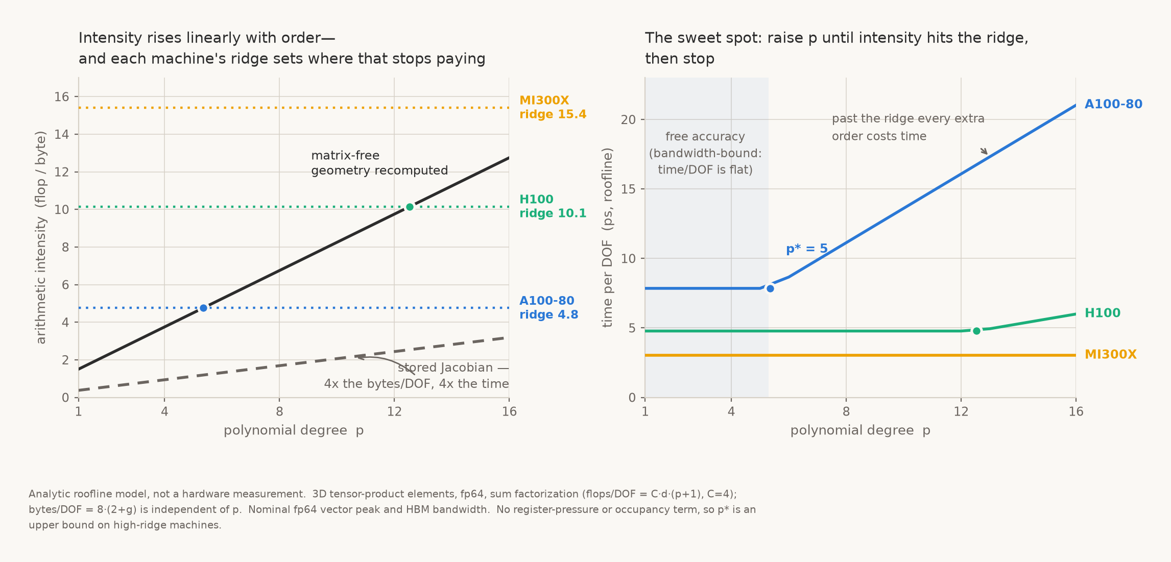
Running the numbers with C = 4, d = 3, recomputed geometry:

Machine	fp64 peak	HBM bandwidth	Ridge (flop/byte)	Sweet spot p*
A100-80 SXM	9.7 TFLOP/s	2039 GB/s	4.8	≈ 5
H100 SXM5	34 TFLOP/s	3350 GB/s	10.1	≈ 12
MI300X	81.7 TFLOP/s	5300 GB/s	15.4	≈ 19

Three things fall out of the model. Read them as predictions; the next section tests them.

The sweet spot is real and it is low. On an A100 the model puts p* ≈ 5. That is a sanity check worth noticing: the CEED and libCEED bake-off campaigns find peak matrix-free throughput empirically in the range p ≈ 5–8, arrived at by measurement rather than by this back-of-the-envelope.

Recompute rather than fetch, quantified. Storing the Jacobian instead of recomputing it quadruples bytes per DOF, which quarters the arithmetic intensity — and if the kernel is bandwidth-bound, where time/DOF = bytes/DOF ÷ bandwidth, it quadruples the time per DOF outright. Note the conditional; it will matter.

The sweet spot moves up with each hardware generation. Ridge points rise — 4.8 on A100, 10.1 on H100, 15.4 on MI300X — because peak FLOP/s has grown faster than bandwidth. So the optimal polynomial order should rise with the hardware, and the discretization you choose is a function of the machine you run it on.

One more number explains why matrix-free is the only way this game can be played at all. An assembled sparse matvec reads roughly eight bytes of matrix per two flops, so its arithmetic intensity is about 0.25 flop/byte — constant, no matter what p you choose. It cannot be moved. Worse, its storage grows as (p+1)^d bytes per DOF: at p = 16 that is roughly 39 kB per degree of freedom. Matrix-free at the same order sits at 12.75 flop/byte on 16 bytes per DOF — a 51× intensity advantage, achieved by not storing the operator. Assembly is what pins you to the bandwidth-bound floor; sum factorization is what lets you climb.

The model carries no term for register pressure, shared-memory working set, or occupancy — all of which bite. The constant C is a stand-in for an implementation-specific flop count; halving it doubles p*. That single soft spot turns out to matter more than everything else.

The model is thirty lines and every assumption is in the header: ai_sweep.py reproduces the tables above, including the sensitivity of p* to C and g, and make_fig.py draws the figure.

Then I rented an A100 and measured it

The model cost nothing and the experiment cost about $2.30 — an hour and a half on a rented A100-SXM4-80GB. I wrote a matrix-free tensor-product Laplacian apply in CUDA (fp64, sum factorization, one element per thread block), swept the degree p = 1…9, measured this specific card's own peaks rather than trusting a datasheet, and used Nsight Compute to count flops, DRAM bytes, and where the time actually went. The card's measured peaks: 7.74 TFLOP/s fp64 and 1752 GB/s triad bandwidth, giving a measured ridge of 4.42 flop/byte (the model had assumed 4.76 from nominal specs — close enough).

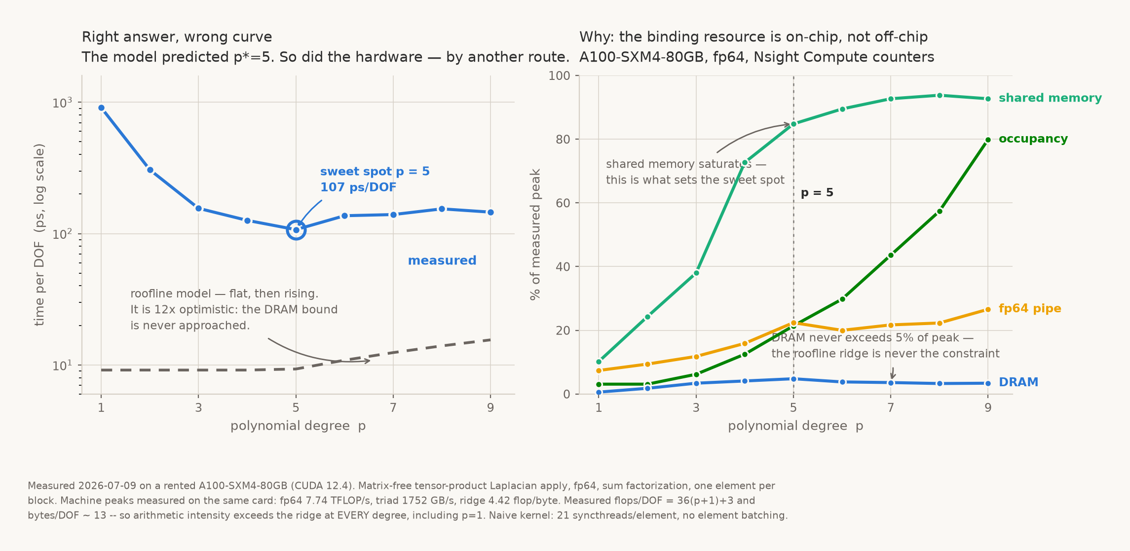
The measured sweet spot is exactly p = 5, at 107 ps/DOF. The model's headline number was right.

Everything else about the model was wrong.

The DRAM roofline never binds — anywhere. Measured flops/DOF came out at 36(p+1)+3, three times the model's 12(p+1): the real Laplacian does eighteen one-dimensional contractions, not six. Measured bytes/DOF is about 13 (the model said 16). So the true arithmetic intensity is ≈ 2.8(p+1), which already exceeds the 4.42 ridge at p = 1 and reaches 16.8 flop/byte at p = 5 — nearly four times above the ridge. There is no bandwidth-bound regime to sit in. The flat region the model drew does not exist.

Two errors cancelled. Underestimating the flop count by 3× pushed the model's fake ridge crossing from p ≈ 1 out to p ≈ 5, which happens to be where the real optimum lives. The model was right by luck.

So what does set the sweet spot? The counters answer without ambiguity. At p = 5 the kernel runs at 5% of DRAM peak, 22% of fp64 peak, and 85% of shared-memory throughput. The binding resource is on-chip. Below p = 5 the kernel is starved — at p = 1 a thread block is 8 threads and occupancy is 3%, so time per DOF is 911 ps, nine times worse than the optimum, for reasons that have nothing to do with bandwidth or flops. Above p = 5 shared memory saturates past 90% and the temporaries stop fitting comfortably. The minimum sits where the block is finally big enough to fill a warp scheduler and not yet big enough to choke the shared-memory pipe.

And so the model's other two predictions collapse:

• "Storing the Jacobian quadruples time/DOF" — false for this kernel. That conclusion assumed a bandwidth-bound regime that does not occur. At 5% of DRAM peak, quadrupling DRAM traffic would be nearly free. Recompute rather than fetch is still good advice, but not for the reason the model gave.
• "The sweet spot rises with each hardware generation" — unsupported. It was derived entirely from rising ridge points, and the ridge is not what selects p. Whether p* moves on an H100 now depends on shared-memory bandwidth and occupancy limits, which I did not measure. I would have to rent an H100 to say, and I have not.

What survives is stronger for having been tested: for matrix-free high-order operator apply, bytes/DOF is small and constant, so arithmetic intensity is above the ridge from p = 1 onward, and the DRAM roofline can never be the thing that picks your polynomial order. The sweet spot is real, it is near p = 5, and it is decided on-chip.

The honest limits of the measurement, in turn. This is one naive kernel: one element per block, twenty-one __syncthreads per element, no batching of small elements, no register-resident temporaries. Production implementations (libCEED, deal.II, MFEM) do all of those things, and would shift both the depth and the location of the minimum — the low-p collapse in particular is largely an artifact of my one-element-per-block choice, which a real code avoids by packing several elements into one block. Single run, single card, no repeats or error bars. What I claim is what I measured: this kernel, on this A100, has its optimum at p = 5 and is shared-memory-bound there.

The kernel, the peak microbenchmarks, and the raw Nsight counters are published: bench.cu · peak.cu · sweep.txt · raw.csv · peaks.txt · make_fig_measured.py

There is a lesson here beyond polynomial orders, and it is the one this whole site keeps circling. A roofline model is a bound, not a prediction. It tells you what the machine cannot exceed; it does not tell you what your kernel will do, and when a kernel runs at 5% of the bound the model was never describing the kernel at all. The model agreed with the measurement on the one number I could check against the literature, which is exactly the circumstance in which a wrong model is most dangerous — it looks validated. The only thing that caught it was going and measuring where the time went. That is what performance engineers deal in: measured ground truth, not plausible arithmetic.

And this is where dataflow architectures point

The argument sharpens on spatial and dataflow machines. Those designs stream operands through a fabric of compute elements and reward reuse in place; they penalize irregular gather/scatter and global synchronization far more than a GPU does. Structured, matrix-free, high-order kernels — small dense tensor contractions on a static dependency graph — are close to the ideal workload for such a fabric. What maps badly is precisely the irregular part of multigrid: an algebraic hierarchy with data-dependent sparsity and shrinking, latency-dominated coarse levels.

The prediction, offered as reasoning rather than measurement, is that these machines widen the gap between geometric, high-order, matrix-free multigrid and classical algebraic multigrid — and that the co-design question stops being "how do I fit my hierarchy on this device" and becomes "which discretization should I have chosen so the hierarchy is regular in the first place." That is a pre-silicon question, and it is the reason the math and the architecture have to be designed together.

The wider pattern: what else cheap arithmetic brought back

Multigrid is one instance of a general rehabilitation. A whole class of methods grounded in matrix theory was priced out when arithmetic was expensive, and is being repriced now. Each trades arithmetic for something scarcer — memory traffic, passes over data, synchronization, or storage:

• High-order spectral-element and discontinuous-Galerkin discretizations — many more flops per degree of freedom, far fewer degrees of freedom for a given accuracy, and much higher arithmetic intensity.
• Hierarchical low-rank methods — fast multipole, H-matrices, hierarchical semi-separable factorizations: O(N) or O(N log N) at the cost of heavy arithmetic and tree traversal.
• Randomized numerical linear algebra — sketching and randomized range finders spend extra flops to cut the number of passes over a matrix that does not fit in memory.
• Mixed-precision iterative refinement — low-precision factorization plus a refinement loop, now the standard route to tensor-core throughput without surrendering accuracy.
• Krylov methods with many matrix-vector products — s-step and communication-avoiding variants, exponential integrators, Chebyshev-filtered subspace iteration for eigenproblems.
• Low-rank tensor formats (tensor-train, hierarchical Tucker) and sparse-grid combination techniques — arithmetic-heavy routes around the curse of dimensionality.
• Monte Carlo and quasi-Monte Carlo for high-dimensional PDEs, and lattice Boltzmann for flow: embarrassingly parallel, arithmetic-hungry, memory-local.

The unifying rule is the same one that rehabilitated the Chebyshev smoother: recompute rather than fetch; do redundant work rather than communicate. An algorithm's FLOP count is no longer its cost. Its arithmetic intensity and its synchronization count are.

The through-line: the theory tells you the O(N) ceiling and names the exact trades — smoother strength against parallelism, cycle depth against occupancy, polynomial order against arithmetic intensity. What the hardware decides is which trade is currently the cheap one. That is what makes the math worth knowing before you write a kernel, and it is why a method invented in 1977 is a better fit for a 2026 accelerator than it was for the machine it was designed on.

What multigrid teaches a loss function

Training minimizes a loss L(θ). A discretized PDE and a loss landscape are both multiscale objects, and the multigrid picture transfers — but it transfers with a twist that is more interesting than a clean analogy would be.

The spectrum runs the other way. A relaxation sweep on a PDE kills high frequencies first and stalls on the smooth ones. Gradient descent on a neural network does the opposite: it fits low-frequency structure first and high-frequency detail last. This is the spectral bias result of Rahaman et al., and it is the reason that coordinate-based networks need help — Fourier features and positional encodings exist to lift high-frequency content into a range where gradient descent can see it. The point is not that a network is a smoother. It is that both objects have a characterized error spectrum, and in both cases naming the spectrum tells you which fix is principled rather than lucky.

The V-cycle generalizes to optimization. Multilevel optimization — MG/OPT, due to Nash — applies the multigrid recursion to a minimization problem directly. Build a hierarchy of coarse models: fewer parameters, downsampled inputs, shorter sequences. Take cheap steps on the coarse model to correct the smooth component of the parameter error, prolong the correction back to the fine model, and smooth with ordinary fine-level steps. The informal versions of this are everywhere in practice — coarse-to-fine training schedules, progressive growing, multi-resolution curricula — usually adopted empirically and rarely recognized as a V-cycle.

Three places multigrid has actually landed in deep learning. These are not analogies; they are published methods, and they enter at three different levels of the stack:

• In the architecture. Ke, Maire & Yu's Multigrid Neural Architectures runs network layers across a pyramid of grids rather than a single spatial grid, with filters carrying both within-scale and cross-scale extent. Receptive field then grows exponentially with depth, and the network learns attention-like behavior that a flat-grid CNN does not.
• In the operator. He & Xu's MgNet is the rigorous version: an explicit correspondence between the steps of a classical multigrid cycle and the operators of a convolutional network — smoothing becomes convolution, restriction becomes pooling — which makes a CNN and a V-cycle two readings of the same object.
• In the training schedule. Wu, Girshick, He, Feichtenhofer & Krähenbühl's A Multigrid Method for Efficiently Training Video Models varies the mini-batch shape on a schedule of coarse-to-fine sampling grids, scaling batch size so that per-batch FLOPs stay roughly constant. Coarse grids early let SGD sweep the dataset cheaply; fine grids late recover accuracy. On Kinetics-400 this trains a SlowFast ResNet-50 about 4.5× faster in wall-clock time while gaining 0.8% top-1 accuracy, out of the box, across models, datasets, and hardware from 1 to 128 GPUs.

That last result is worth pausing on, because it is the cheap-arithmetic argument of the previous section pointed at training. The grid schedule holds FLOPs per mini-batch fixed and rearranges them — more examples at low resolution early, fewer at high resolution late. The speedup does not come from doing less arithmetic. It comes from spending the same arithmetic where the optimizer can use it, which is exactly what a coarse-grid correction does for a linear solve.

Multigrid in time. Sequential dependency is a parallelism killer: backpropagation through time, long autoregressive rollouts, and time-stepped simulation all serialize. Parallel-in-time methods (parareal, and MGRIT, which is literally multigrid applied to the time axis) build a coarse temporal grid, solve it cheaply, and use it to correct fine-grid time steps computed in parallel. It is the same complementarity argument, with time as the dimension being coarsened.

As a preconditioner. Second-order and natural-gradient optimizers require solving a linear system in a curvature operator each step. When that operator is elliptic-like, multigrid is the right inner solver, and the outer optimizer inherits its mesh-independence.

A caution, since the analogy is seductive: these are not the same theorem. The O(N) result rests on properties of an elliptic operator — a spectrum you can characterize, a coarse space that provably approximates the smooth error. A loss landscape is nonconvex, and a "coarse model" is not a Galerkin projection of a fine one in any rigorous sense. MgNet earns its correspondence at the level of operators; the video-training result earns its 4.5× empirically, and its authors are explicit that they take multigrid "from a more abstract view" rather than inheriting its convergence theory. So there is no mesh-independence guarantee waiting for you at the end of a coarse-to-fine training schedule, and none of these methods claims one.

What transfers is the reasoning, not the guarantee — and the reasoning has been load-bearing enough to produce a 4.5× speedup and an accuracy gain at 128-GPU scale. That is the useful state to hold: the mathematics is a source of correct questions about where an optimizer's error lives, not a source of theorems about where it goes.

The one-line version

Multigrid is the mathematics of matching a solver to the frequency content of the error, across scales. Cheap local steps for fine detail; coarse global steps for smooth structure; neither sufficient alone. Once you have that frame, you notice it everywhere — in an elliptic solve, in a training schedule, in a parallel-in-time integrator.

And the second lesson, which took the hardware fifty years to teach: an algorithm's cost is not its FLOP count. Multigrid was designed under a cost model that no longer holds, and it is better now than it was then — not because anyone improved the theory, but because the machine finally began charging for the thing the theory was quietly economizing. The components once dismissed as wasteful are the ones that run fast. Knowing which resource is scarce is not a detail of implementation. It is the algorithm-selection problem.

It is structure is knowledge in its oldest form. The structure here is a spectrum, and knowing it buys you an algorithm with a provable ceiling — which, unlike most things in performance engineering, you can check your implementation against rather than merely hoping you have not left something on the table. It is also the counterweight to the argument in what a PINN is and is not: a PINN turns a PDE into a loss function and pays four to five orders of magnitude for the privilege, and the reason the mesh wins so decisively is that seventy years of numerical analysis — multigrid chief among it — went into making the mesh solve optimal.

References

1. A. Brandt, Multi-Level Adaptive Solutions to Boundary-Value Problems, Math. Comp. 31 (1977), 333–390.
2. W. L. Briggs, V. E. Henson, S. F. McCormick, A Multigrid Tutorial, 2nd ed., SIAM, 2000.
3. U. Trottenberg, C. Oosterlee, A. Schüller, Multigrid, Academic Press, 2001.
4. J. W. Ruge, K. Stüben, Algebraic Multigrid, in Multigrid Methods (S. McCormick, ed.), SIAM, 1987.
5. A. H. Baker, R. D. Falgout, T. V. Kolev, U. M. Yang, Multigrid Smoothers for Ultraparallel Computing, SIAM J. Sci. Comput. 33 (2011).
6. S. G. Nash, A Multigrid Approach to Discretized Optimization Problems, Optim. Methods Softw. 14 (2000), 99–116.
7. N. Rahaman et al., On the Spectral Bias of Neural Networks, ICML 2019: https://arxiv.org/abs/1806.08734
8. M. Tancik et al., Fourier Features Let Networks Learn High Frequency Functions in Low Dimensional Domains, NeurIPS 2020: https://arxiv.org/abs/2006.10739
9. R. D. Falgout, S. Friedhoff, T. V. Kolev, S. P. MacLachlan, J. B. Schroder, Parallel Time Integration with Multigrid, SIAM J. Sci. Comput. 36 (2014).
10. J.-L. Lions, Y. Maday, G. Turinici, Résolution d'EDP par un schéma en temps «pararéel», C. R. Acad. Sci. Paris 332 (2001).

Multigrid and deep learning

1. T.-W. Ke, M. Maire, S. X. Yu, Multigrid Neural Architectures, CVPR 2017. DOI 10.1109/CVPR.2017.433 · https://arxiv.org/abs/1611.07661
2. J. He, J. Xu, MgNet: A Unified Framework of Multigrid and Convolutional Neural Network, Science China Mathematics 62 (2019). DOI 10.1007/s11425-019-9547-2
3. C.-Y. Wu, R. Girshick, K. He, C. Feichtenhofer, P. Krähenbühl, A Multigrid Method for Efficiently Training Video Models, CVPR 2020: https://arxiv.org/abs/1912.00998

Trading arithmetic for bandwidth, passes, and synchronization

1. M. Kronbichler, K. Kormann, A Generic Interface for Parallel Cell-Based Finite Element Operator Application, Computers & Fluids 63 (2012), 135–147. (Matrix-free sum factorization.)
2. E. Carson, N. J. Higham, Accelerating the Solution of Linear Systems by Iterative Refinement in Three Precisions, SIAM J. Sci. Comput. 40 (2018), A817–A847.
3. N. Halko, P. G. Martinsson, J. A. Tropp, Finding Structure with Randomness, SIAM Review 53 (2011), 217–288. (Randomized numerical linear algebra.)
4. L. Greengard, V. Rokhlin, A Fast Algorithm for Particle Simulations, J. Comput. Phys. 73 (1987), 325–348. (Fast multipole.)
5. M. Hoemmen, Communication-Avoiding Krylov Subspace Methods, Ph.D. thesis, UC Berkeley, 2010.
6. A. George, Nested Dissection of a Regular Finite Element Mesh, SIAM J. Numer. Anal. 10 (1973), 345–363. (The sparse-direct fill-in complexity.)